Common Agricultural Experimental Designs with speed

Introduction

Agricultural experiments require careful spatial design to minimise the effects of field heterogeneity and neighbour interactions while maximising statistical power. The speed package provides tools for creating spatially efficient experimental designs through simulated annealing optimisation.

This vignette demonstrates how to use speed for common agricultural experimental designs, showing how spatial optimisation can improve the efficiency and validity of field trials. We’ll work through four key design types, each building in complexity and showing different features of the package.

library(speed)

Completely Randomised Design (CRD)

Overview

The Completely Randomised Design is the simplest experimental design where treatments are assigned to experimental units entirely at random. While simple to implement, CRD doesn’t account for spatial variation in field conditions.

When to Use

Homogeneous experimental conditions
Controlled environments (greenhouse, growth chamber)
Small-scale experiments with minimal spatial variation
Proof-of-concept studies

Example: Field Trial with 8 Varieties

Consider a field trial testing 8 new wheat varieties with 4 replicates each. Even though treatments are assigned randomly, spatial optimization can reduce neighbor effects and improve precision.

Setting Up CRD with speed

In agricultural contexts, even completely randomised designs benefit from spatial optimisation to minimise treatment clustering and neighbour effects. Firstly we will initialise a dataframe representing the design and visualise it. This design has 4 replicates of 8 treatments or items, with 8 rows and 4 columns.

# Initialise dataframe
crd_design <- initialise_design_df(items = 8, nrows = 8, ncols = 4)
head(crd_design)

  row col treatment
1   1   1        T1
2   2   1        T2
3   3   1        T3
4   4   1        T4
5   5   1        T5
6   6   1        T6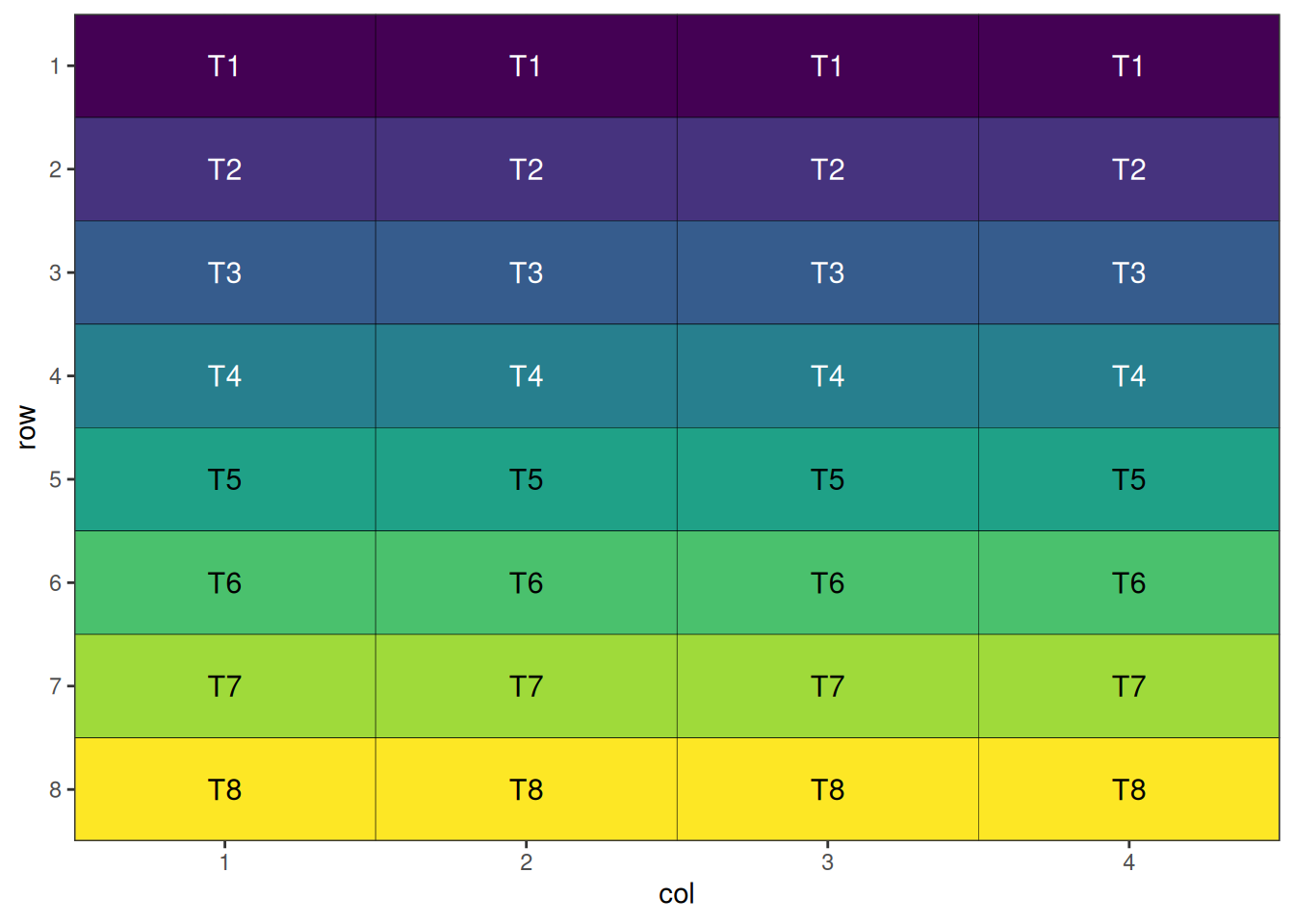

This is a systematic layout; note how the initial layout arranges treatments in a repeating, non-random pattern. This will now be randomised before visualisation.

Performing the Optimisation

The main speed() function performs the optimisation. It has been set up with sensible defaults to allow application to a wide variety of situations. In this case, we only need to provide the design dataframe for it to operate on, the column name of the dataframe to use for the treatments, and a seed for reproducibility.

crd_result <- speed(crd_design, 
                    swap = "treatment",
                    seed = 42)

row and col are used as row and column, respectively.

Iteration: 1000 Score: 2.285714 Best: 2.285714 Since Improvement: 271
Iteration: 2000 Score: 2.285714 Best: 2.285714 Since Improvement: 1271
Early stopping at iteration 2729

crd_result

Optimised Experimental Design
----------------------------
Score: 2.285714
Iterations Run: 2730
Stopped Early: TRUE
Treatments: T1, T2, T3, T4, T5, T6, T7, T8
Seed: 42

Output of the Optimisation

The printed output from the returned design object shows the final optimisation score (lower is better), the number of iterations taken to reach that result, if the iterations stopped early due to lack of improvement, the treatments present in the design, and the seed. The output object contains some additional components, which can be seen below:

str(crd_result)

List of 8
 $ design_df     :Classes 'design' and 'data.frame':    32 obs. of  3 variables:
  ..$ row      : int [1:32] 1 1 1 1 2 2 2 2 3 3 ...
  ..$ col      : int [1:32] 1 2 3 4 1 2 3 4 1 2 ...
  ..$ treatment: chr [1:32] "T8" "T1" "T7" "T3" ...
 $ score         : num 2.29
 $ scores        : num [1:2730] 40 36.3 32.4 28.3 24.1 ...
 $ temperatures  : num [1:2730] 100 99 98 97 96.1 ...
 $ iterations_run: int 2730
 $ stopped_early : logi TRUE
 $ treatments    : chr [1:8] "T1" "T2" "T3" "T4" ...
 $ seed          : num 42
 - attr(*, "class")= chr [1:2] "design" "list"

Visualise the Output

The final step is to visualise the optimised design. The plot below displays the spatial arrangement of treatments after optimisation, allowing you to easily check for clustering, spatial trends, or other patterns that may affect your experiment. A well-randomised and spatially efficient design will show treatments distributed evenly across the field, helping to minimise neighbour effects and maximise the reliability of your results.

autoplot(crd_result)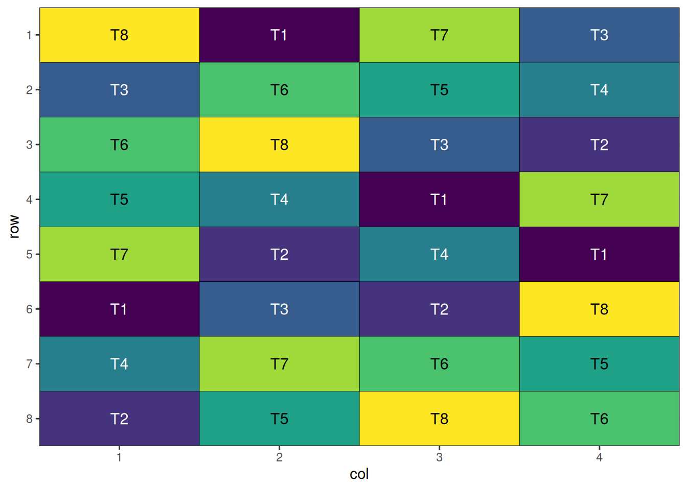

A nicely randomised and spatially optimal design!

Randomised Complete Block Design (RCBD)

Overview

RCBD is one of the most commonly used designs in agricultural research. It controls for one source of variation by grouping experimental units into homogeneous blocks, with each treatment appearing once per block.

When to Use

Field experiments with known gradient (slope, soil type, irrigation)
Medium to large experiments (3+ treatments)
When blocking factor explains significant variation
Multi-location trials

Example: Variety Trial Across Field Gradient

Consider testing 6 soybean varieties across a field with a moisture gradient. Using 4 blocks perpendicular to the gradient helps control for soil moisture variation.

Setting Up RCBD with speed

Here we initialise a dataframe for a design with 4 blocks and 6 treatments, arranged in 4 rows and 6 columns. Note that we can specify treatments in the items argument.

rcbd_design <- initialise_design_df(items = paste0("V", 1:6), nrows = 4, ncols = 6, block_nrows = 1, block_ncols = 6)
head(rcbd_design)

  row col treatment row_block col_block block
1   1   1        V1         1         1     1
2   2   1        V2         2         1     2
3   3   1        V3         3         1     3
4   4   1        V4         4         1     4
5   1   2        V5         1         1     1
6   2   2        V6         2         1     2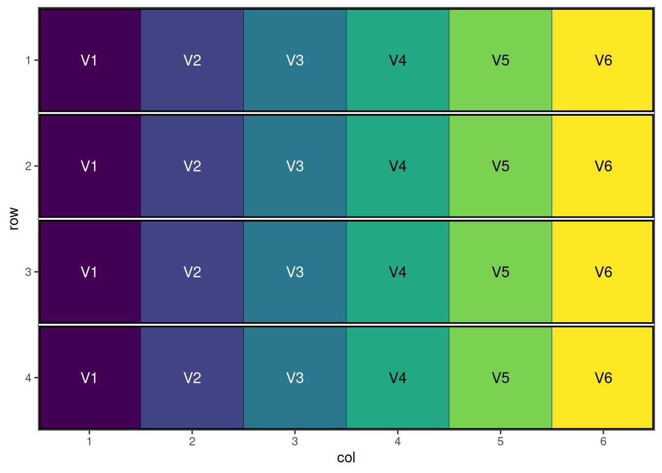

This is a systematic block layout; each block contains all treatments in a repeating pattern. This will now be randomised within blocks.

Performing the Optimisation

rcbd_result <- speed(rcbd_design, 
                     swap = "treatment",
                     swap_within = "block",
                     seed = 42)

row and col are used as row and column, respectively.

Iteration: 1000 Score: 1.6 Best: 1.6 Since Improvement: 672
Iteration: 2000 Score: 1.6 Best: 1.6 Since Improvement: 1672
Early stopping at iteration 2328

rcbd_result

Optimised Experimental Design
----------------------------
Score: 1.6
Iterations Run: 2329
Stopped Early: TRUE
Treatments: V1, V2, V3, V4, V5, V6
Seed: 42

Output of the Optimisation

str(rcbd_result)

List of 8
 $ design_df     :Classes 'design' and 'data.frame':    24 obs. of  6 variables:
  ..$ row      : int [1:24] 1 1 1 1 1 1 2 2 2 2 ...
  ..$ col      : int [1:24] 1 2 3 4 5 6 1 2 3 4 ...
  ..$ treatment: chr [1:24] "V4" "V1" "V5" "V6" ...
  ..$ row_block: int [1:24] 1 1 1 1 1 1 2 2 2 2 ...
  ..$ col_block: int [1:24] 1 1 1 1 1 1 1 1 1 1 ...
  ..$ block    : num [1:24] 1 1 1 1 1 1 2 2 2 2 ...
 $ score         : num 1.6
 $ scores        : num [1:2329] 34 29.6 25.2 21.6 18.4 16.2 13 12.2 8.6 10.4 ...
 $ temperatures  : num [1:2329] 100 99 98 97 96.1 ...
 $ iterations_run: int 2329
 $ stopped_early : logi TRUE
 $ treatments    : chr [1:6] "V1" "V2" "V3" "V4" ...
 $ seed          : num 42
 - attr(*, "class")= chr [1:2] "design" "list"

Visualise the Output

autoplot(rcbd_result)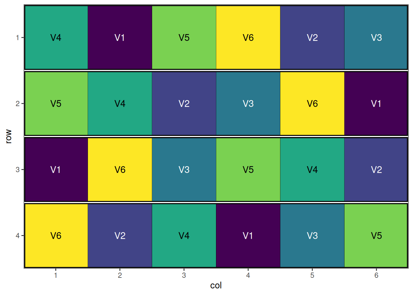

A well-randomised and spatially efficient RCBD layout.

Latin Square Design

Overview

Latin Square Design controls for two sources of variation simultaneously by arranging treatments in a square grid where each treatment appears exactly once in each row and column.

When to Use

Small to medium experiments (3-10 treatments)
Two known sources of variation (e.g., row and column effects)
Greenhouse bench experiments
Field experiments with two-way gradients

Constraints

Number of treatments must equal number of rows and columns
Limited degrees of freedom for error
Assumes no row × column interaction

Setting Up Latin Square with speed

Here we initialise a 5 × 5 Latin square with 5 treatments.

latin_square_design <- initialise_design_df(items = 5, nrows = 5, ncols = 5)
head(latin_square_design)

  row col treatment
1   1   1        T1
2   2   1        T2
3   3   1        T3
4   4   1        T4
5   5   1        T5
6   1   2        T1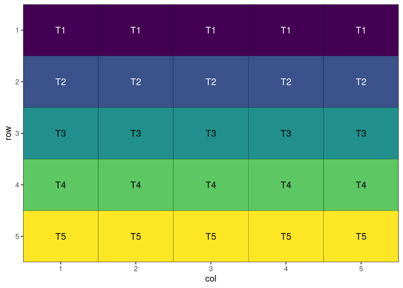

This is a systematic Latin square layout; each treatment appears once per row and column. The design will now be randomised.

Performing the Optimisation

Because of the spatial optimisation algorithm built into speed, with default options and enough iterations, it should arrive at a Latin square design in cases where the number of rows, columns, treatments and replicates are all equal such as this.

latin_square_result <- speed(latin_square_design, 
                             swap = "treatment",
                             seed = 42)

row and col are used as row and column, respectively.

Iteration: 1000 Score: 1 Best: 1 Since Improvement: 308
Early stopping at iteration 1040

latin_square_result

Optimised Experimental Design
----------------------------
Score: 0
Iterations Run: 1041
Stopped Early: TRUE
Treatments: T1, T2, T3, T4, T5
Seed: 42

Output of the Optimisation

Note that the final score of zero shows that the algorithm has found a perfect Latin Square solution.

str(latin_square_result)

List of 8
 $ design_df     :Classes 'design' and 'data.frame':    25 obs. of  3 variables:
  ..$ row      : int [1:25] 1 1 1 1 1 2 2 2 2 2 ...
  ..$ col      : int [1:25] 1 2 3 4 5 1 2 3 4 5 ...
  ..$ treatment: chr [1:25] "T3" "T2" "T5" "T1" ...
 $ score         : num 0
 $ scores        : num [1:1041] 45 39 37 33.5 30.5 32.5 32 30.5 26.5 29 ...
 $ temperatures  : num [1:1041] 100 99 98 97 96.1 ...
 $ iterations_run: int 1041
 $ stopped_early : logi TRUE
 $ treatments    : chr [1:5] "T1" "T2" "T3" "T4" ...
 $ seed          : num 42
 - attr(*, "class")= chr [1:2] "design" "list"

Visualise the Output

autoplot(latin_square_result)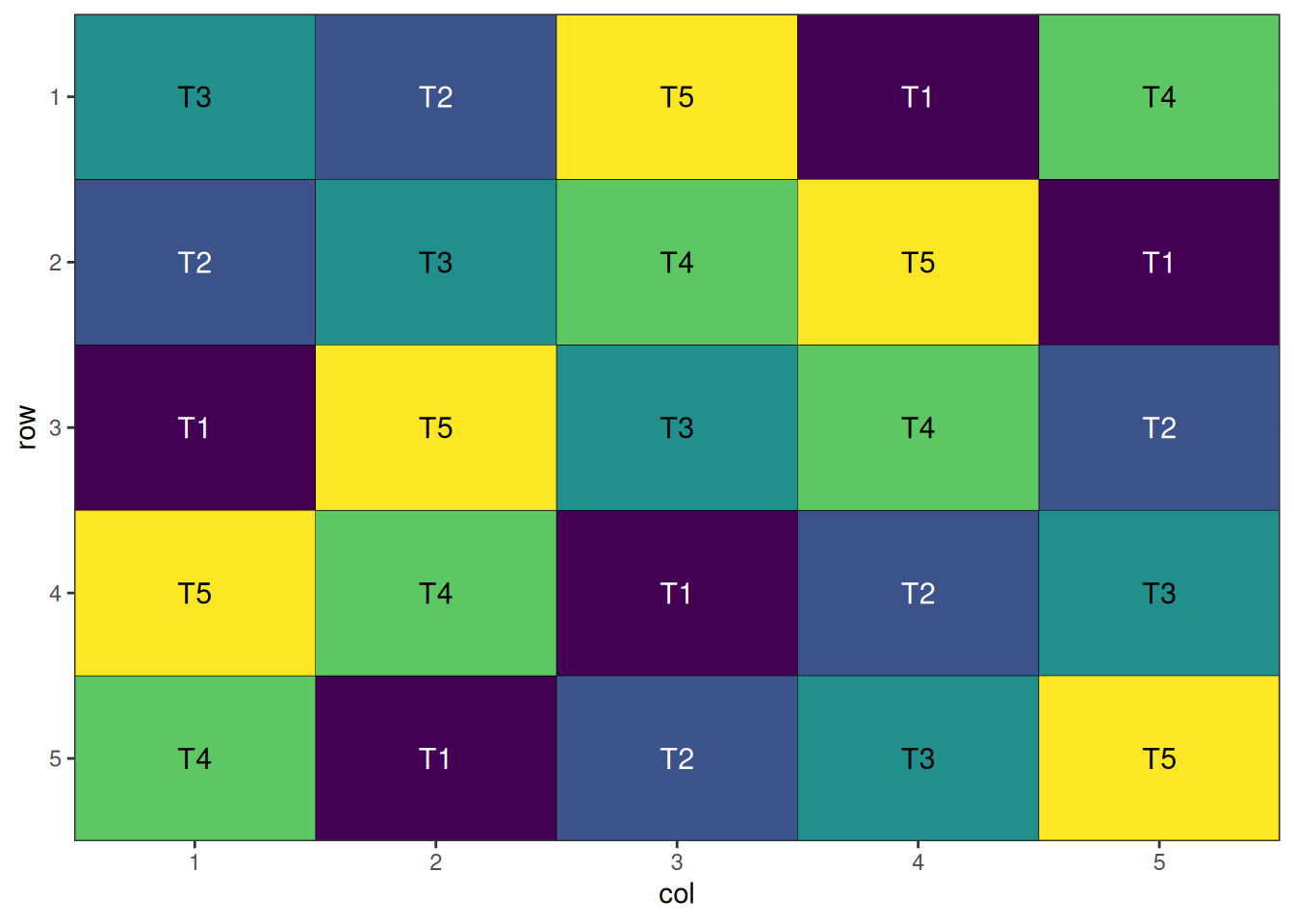

A well-randomised and spatially efficient Latin square layout.

Split-Plot Design

Overview

Split-Plot Design is used when some treatments are easier to apply to large areas (whole plots) while others require smaller areas (sub-plots). This creates a hierarchical structure with different levels of precision. Split-Plot Designs are particularly useful in agricultural experiments where some factors are difficult or expensive to replicate at the whole plot level. These designs are possible with the speed package, allowing for spatial optimisation of both whole plots and sub-plots in a single step.

When to Use

Treatments with different application scales (large vs small plots)
Irrigation × variety experiments
Tillage × fertilizer studies
When some treatments are expensive or difficult to replicate

Structure

Whole plots: Larger experimental units (main treatments)
Sub-plots: Smaller units within whole plots (sub-treatments)
Different error terms for different treatment levels

Setting Up Split Plot Design with speed

Now we can create a dataframe representing a split plot design. Note that the initalise_design_df function does not currently support split plot designs directly, so we will create it manually.

split_plot_design <- data.frame(
    row = rep(1:12, each = 4),
    col = rep(1:4, times = 12),
    block = rep(1:4, each = 12),
    wholeplot = rep(1:12, each = 4),
    wholeplot_treatment = rep(rep(LETTERS[1:3], each = 4), times = 4),
    subplot_treatment = rep(letters[1:4], 12)
 )
head(split_plot_design)

  row col block wholeplot wholeplot_treatment subplot_treatment
1   1   1     1         1                   A                 a
2   1   2     1         1                   A                 b
3   1   3     1         1                   A                 c
4   1   4     1         1                   A                 d
5   2   1     1         2                   B                 a
6   2   2     1         2                   B                 b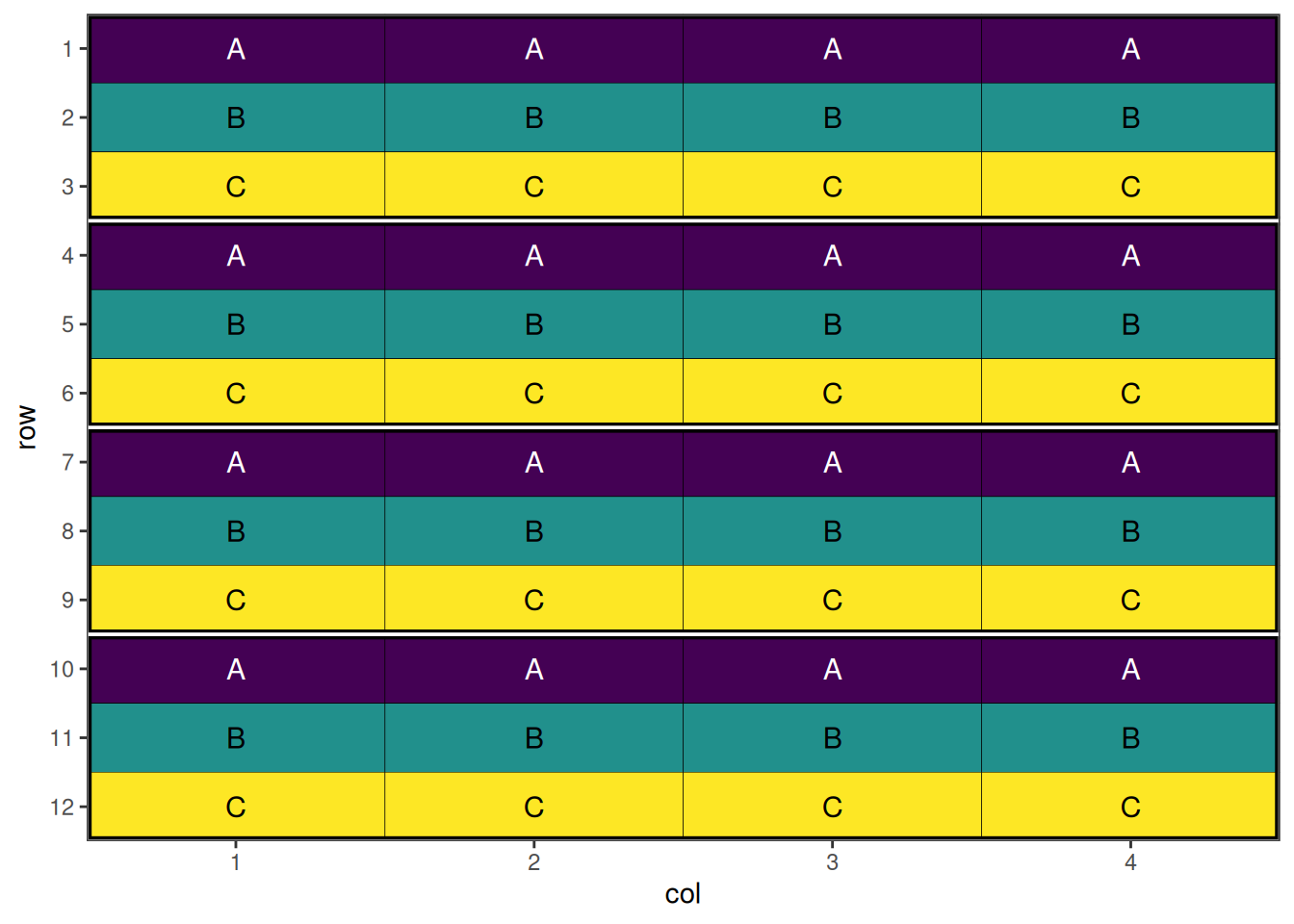

This is a systematic split plot layout; each treatment appears once per block for wholeplot treatments, and once per whole plot for sub-plot treatments. The design will now be randomised.

Performing the Optimisation

For split-plot designs, we use named lists to specify the hierarchical structure. The swap parameter defines what to optimize at each level, while swap_within defines the constraints for each level.

split_plot_result <- speed(split_plot_design,
                           swap = list(wp = "wholeplot_treatment",
                                       sp = "subplot_treatment"),
                           swap_within = list(wp = "block", sp = "wholeplot"),
                           seed = 42)

row and col are used as row and column, respectively.

Optimising level: wp
Level: wp Iteration: 1000 Score: 100 Best: 100 Since Improvement: 1000
Level: wp Iteration: 2000 Score: 100 Best: 100 Since Improvement: 2000
Early stopping at iteration 2000 for level wp
Optimising level: sp
Early stopping at iteration 570 for level sp

split_plot_result

Optimised Experimental Design
----------------------------
Score: 100
Iterations Run: 2572
Stopped Early: TRUE TRUE
Treatments:
  wp: A, B, C
  sp: a, b, c, d
Seed: 42

Output of the Optimisation

The output shows optimization results for the design. The score and iterations are combined for the entire design, while the treatments, and stopping criteria are reported separately for each level, allowing you to assess the quality of optimization at each hierarchy level.

str(split_plot_result)

List of 8
 $ design_df     :Classes 'design' and 'data.frame':    48 obs. of  6 variables:
  ..$ row                : int [1:48] 1 1 1 1 2 2 2 2 3 3 ...
  ..$ col                : int [1:48] 1 2 3 4 1 2 3 4 1 2 ...
  ..$ block              : int [1:48] 1 1 1 1 1 1 1 1 1 1 ...
  ..$ wholeplot          : int [1:48] 1 1 1 1 2 2 2 2 3 3 ...
  ..$ wholeplot_treatment: chr [1:48] "C" "C" "C" "C" ...
  ..$ subplot_treatment  : chr [1:48] "a" "b" "c" "d" ...
 $ score         : num 100
 $ scores        :List of 2
  ..$ wp: num [1:2001] 100 104 104 104 104 104 104 104 100 100 ...
  ..$ sp: num [1:571] 188 169 151 133 125 ...
 $ temperatures  :List of 2
  ..$ wp: num [1:2001] 100 99 98 97 96.1 ...
  ..$ sp: num [1:571] 100 99 98 97 96.1 ...
 $ iterations_run: num 2572
 $ stopped_early : Named logi [1:2] TRUE TRUE
  ..- attr(*, "names")= chr [1:2] "wp" "sp"
 $ treatments    :List of 2
  ..$ wp: chr [1:3] "A" "B" "C"
  ..$ sp: chr [1:4] "a" "b" "c" "d"
 $ seed          : num 42
 - attr(*, "class")= chr [1:2] "design" "list"

Visualise the Output

autoplot(split_plot_result, treatments = "wholeplot_treatment")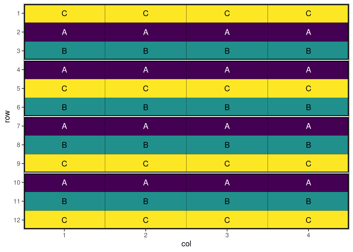

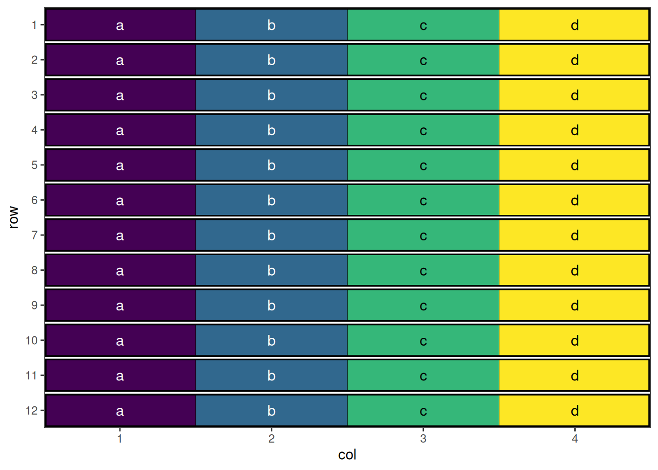
autoplot(split_plot_result, treatments = "subplot_treatment", block = "wholeplot")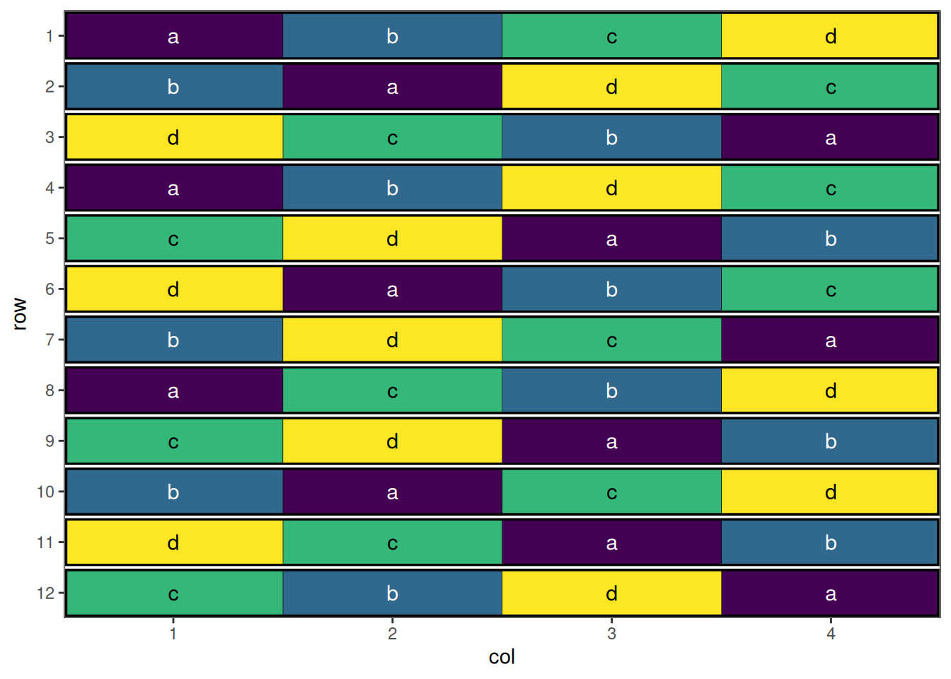

This design has now been optimised at both the whole plot level and the sub-plot level.

Spatial Design Considerations

Field Shape and Orientation

The shape and orientation of your experimental field significantly impacts design efficiency:

Long, narrow fields: Favor designs with blocks perpendicular to the long axis
Square fields: Allow more flexibility in blocking direction
Irregular shapes: May require custom design approaches

Neighbour Effects

Agricultural experiments often experience neighbour effects where adjacent plots influence each other:

Competition effects: Tall varieties shading short ones
Contamination: Fertiliser or pesticide drift
Root competition: Nutrient or water competition between plots

The speed package specifically addresses these issues through spatial optimisation.

Buffer Areas

Consider including buffer areas or border plots to:

Reduce edge effects
minimise contamination between treatments
Provide realistic growing conditions

Using `speed` Effectively

Set appropriate parameters: Balance optimisation time with improvement
Visualise designs: Always plot layouts before implementation
Compare alternatives: Test multiple blocking strategies
Validate results: Check constraint satisfaction and efficiency metrics

Conclusion

The speed package provides powerful tools for creating spatially efficient experimental designs. By optimising treatment arrangements, researchers can:

Reduce neighbour effects and spatial confounding
Improve statistical power and precision
Maintain design validity and balance
Visualise and evaluate design quality

Whether using simple randomised designs or complex split-plot structures, spatial optimisation through speed can significantly enhance the efficiency and reliability of agricultural experiments.

Introduction

Completely Randomised Design (CRD)

Overview

When to Use

Example: Field Trial with 8 Varieties

Setting Up CRD with speed

Performing the Optimisation

Output of the Optimisation

Visualise the Output

Randomised Complete Block Design (RCBD)

Overview

When to Use

Example: Variety Trial Across Field Gradient

Setting Up RCBD with speed

Performing the Optimisation

Output of the Optimisation

Visualise the Output

Latin Square Design

Overview

When to Use

Constraints

Setting Up Latin Square with speed

Performing the Optimisation

Output of the Optimisation

Visualise the Output

Split-Plot Design

Overview

When to Use

Structure

Setting Up Split Plot Design with speed

Performing the Optimisation

Output of the Optimisation

Visualise the Output

Spatial Design Considerations

Field Shape and Orientation

Neighbour Effects

Buffer Areas

Using speed Effectively

Conclusion

Further Reading

Using `speed` Effectively