Pairwise comparisons of predicted means

Test a chosen set of pairwise differences between the predicted means of a fitted model, with multiplicity adjustment over the chosen set and optional splitting into independent subgroups. Unlike multiple_comparisons(), which is means-centric and summarises all pairwise comparisons via a compact letter display, pairwise_comparisons() is difference-centric: it returns a tidy table with one row per requested comparison. This honestly represents selective and irregular comparison sets, for which letter groupings are not valid.

Usage

# S3 method for class 'pairwise_comparisons'
autoplot(object, ..., axis_rotation = 0, label_rotation = 0)

pairwise_comparisons(
  model.obj,
  classify,
  pairs = NULL,
  contrasts = NULL,
  adjust = "holm",
  by = NULL,
  sig = 0.05,
  include_means = TRUE,
  descending = NULL,
  ...
)

# S3 method for class 'pairwise_comparisons'
print(x, decimals = 2, ...)

Arguments

object: A pairwise_comparisons object.
...: Other arguments passed to the model-specific prediction methods (e.g. ASReml-R predict() arguments).
axis_rotation: Rotation (degrees) of the x-axis (estimate) labels.
label_rotation: Rotation (degrees) of the y-axis (comparison) labels.
model.obj: An asreml, aov, lm, lme (nlme::lme()) or lmerMod (lme4::lmer()) model object.
classify: Name of the predictor variable(s) to compare, as a string. Interactions are specified with : (e.g. "Trt:Site").
pairs: The comparisons to test. NULL (default) tests all pairwise comparisons. Otherwise either a character vector of "level1-level2" labels (levels of an interaction joined by :, the two sides of a pair separated by -, e.g. "A:X-B:Y"), or a list of length-2 character vectors (e.g. list(c("A:X", "B:Y"))). Level names may contain -; the list form is only needed if a pair is genuinely ambiguous. See Details.
contrasts: An optional named list of general linear contrasts to test instead of pairs. Each element is a named numeric vector of coefficients keyed by level label (e.g. list("A vs B & C" = c(A = 1, B = -0.5, C = -0.5))), and the list names become the comparison labels. The estimate is the corresponding linear combination of the predicted means. Mutually exclusive with pairs; coefficients should sum to zero (a warning is issued otherwise). include_means does not apply to this form. See Details for how the standard error and degrees of freedom are obtained.
adjust: The method used to adjust p-values for multiplicity over the chosen set, passed to stats::p.adjust(). Default is "holm". Any stats::p.adjust.methods value is accepted. "tukey" is not valid here (it is exact only for the complete set of all pairwise comparisons — use multiple_comparisons() for that).
by: A character vector of one or more classify factors over which to split the comparisons. The same pairs set is tested, and adjusted, independently within each level (or combination of levels) of by, with no pooling across groups. Default NULL. See Details.
sig: The significance level for the confidence intervals, numeric between 0 and 1. Default is 0.05.
include_means: Logical; if TRUE (default) the predicted mean of each side of the comparison is included as level1.mean and level2.mean columns, immediately after estimate. Set FALSE for the differences only.
descending: Tri-state control of row ordering within each by-group. NULL (default) keeps the input order of pairs; FALSE sorts ascending by estimate; TRUE sorts descending by estimate.
x: A pairwise_comparisons object.
decimals: Number of decimal places to display. Default is 2. The p-value is shown to 3 significant figures (rather than rounded) so very small p-values do not collapse to zero.

Value

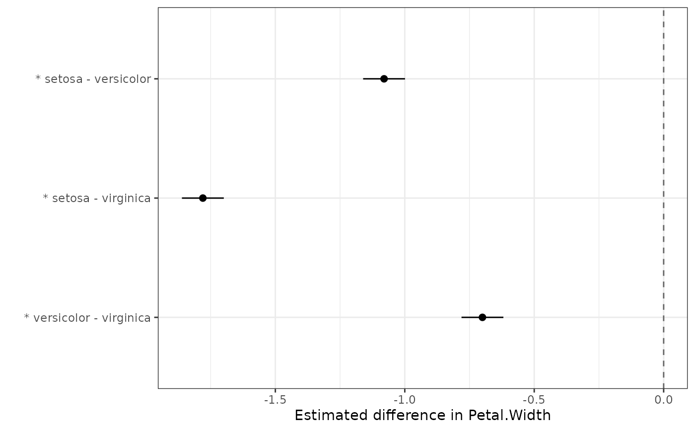
autoplot.pairwise_comparisons() returns a ggplot2 object: a forest plot of the estimated differences with their confidence intervals and a dashed reference line at zero, faceted by the by variable(s) when present. Comparisons that are significant at the adjusted sig level are flagged with an asterisk (*) — prefixed to the y-axis label when unfaceted (keeping the labels right-justified against the axis), or beside the interval when faceted by by.

A data.frame of class pairwise_comparisons with one row per (group × comparison) and columns: any by column(s), level1, level2, comparison, estimate, (optionally level1.mean and level2.mean), std.error, statistic, df, p.value (adjusted), conf.low and conf.high. Stored at full precision; rounding for display is controlled by print.pairwise_comparisons(). For the contrasts form, the level1/level2 and mean columns are omitted and comparison holds the contrast name. If any levels were aliased (not estimable) in the model they are dropped from the comparisons (with a warning) and recorded in an aliased attribute.

print.pairwise_comparisons() invisibly returns x.

Details

Relationship to the other comparison functions

pairwise_comparisons(), multiple_comparisons() and reference_comparisons() share the same predicted means and standard errors of differences; they differ in which comparisons they report. Testing all pairs here (pairs = NULL) with a given adjust yields the same adjusted p-values as multiple_comparisons() with that adjust, while reference_comparisons() is the special case of comparing every level against a single control. Tukey's HSD is exact only for the complete set of all pairwise comparisons, so adjust = "tukey" is not valid for pairwise_comparisons() (use multiple_comparisons()).

`pairs` syntax and sign convention

The estimate for a pair is mean(level1) - mean(level2), in the order written ("A-B" gives A - B). The level1 and level2 columns make the sign unambiguous. With : joining interaction cells and - separating the two sides of a pair, a level name may itself contain -: each - is tried as the separator and the split that yields two valid levels is used (so "A-D-xyz" resolves to A versus D-xyz when those are the real levels). Only when more than one split is valid is the pair genuinely ambiguous, and the list form is then required (the error shows the candidate splits). Reversed or duplicated pairs ("A-B" and "B-A") are de-duplicated with a warning, since duplicates would inflate the adjustment family.

For an interaction classify, the :-joined components of each level label must be in the same order as classify (e.g. "A:X" for classify = "Trt:Site", not "X:A"); the same applies to the level names used in contrasts. A label that names no existing cell is rejected with the list of available levels, but a mis-ordered label that happens to name another valid cell is used silently — so when the factors share level names, check the component order matches classify.

`by` semantics

by must be a subset of the classify factors. Within each group, pair labels reference the remaining (non-by) factor levels. For example, classify = "Trt:Site", by = "Site", pairs = "A-B" compares Trt levels A and B within each Site. A group with fewer than two levels is skipped with a warning. In an unbalanced design a requested comparison may reference a level that is absent from some groups: such a comparison is skipped (with a warning) in the groups where it cannot be computed and reported in those where it can. A level that is absent from every group — or that was aliased — is instead an error, since that indicates a mistake rather than an incomplete design.

Standard error and degrees of freedom for `contrasts`

The contrast variance is c' V c, where V is the variance-covariance matrix of the predicted means taken directly from the fitting engine (no reconstruction). The degrees of freedom depend on the engine:

For models predicted via emmeans (aov, lm, nlme::lme(), lme4::lmer(), and aov with Error() strata) the estimate, standard error and degrees of freedom are obtained directly from emmeans::contrast() on the model's reference grid. The degrees of freedom are therefore the exact contrast df for that engine (Satterthwaite or Kenward-Roger for mixed models, containment for aov/Error()), including for contrasts spanning more than two levels.
For asreml models V is the prediction error covariance from predict(..., vcov = TRUE), and the degrees of freedom are the term's denominator df from asreml::wald(denDF = "default") (a single Kenward-Roger-style value shared by all contrasts within the term, as ASReml-R does not provide a per-contrast approximate df).

Transformations

Comparisons are reported on the model scale. A difference of transformed means does not back-transform to a difference on the original scale (for log/logit it is a ratio), so back-transformation is not attempted; a warning is issued if the response appears to be transformed in the model formula.

Confidence intervals

The per-comparison confidence intervals are not simultaneity-adjusted: as with the confidence-interval/letter note in multiple_comparisons(), an interval may exclude zero while the adjusted p-value is >= sig. When this happens a one-time message() notes it (suppressible with suppressMessages()).

Supported model types

The comparison functions (multiple_comparisons(), pairwise_comparisons() and reference_comparisons()) work with any model for which a get_predictions() method is defined. These are currently:

Model class	Fitted by	Notes
`aov`, `lm`	`stats::aov()`, `stats::lm()`	Fixed-effects linear models.
`aovlist`	`stats::aov()` with an `Error()` term	Multi-stratum aov; gives comparison-specific (matrix) degrees of freedom.
`lme`	`nlme::lme()`	Linear mixed model.
`lmerMod`	`lme4::lmer()`, `lme4breeding::lmebreed()`	Linear mixed model. `lmebreed()` (relationship-based) models also carry class `lmerMod`; comparisons target the fixed-effect means with Kenward-Roger degrees of freedom, and correctly reflect the relationship structure (validated against ASReml-R).
`lmerModLmerTest`	`lmerTest::lmer()`	As `lmerMod`, with Satterthwaite degrees of freedom.
`asreml`	ASReml-R `asreml()`	Linear mixed model (commercial; not on CRAN).
`afex_aov`	afex `aov_car()` / `aov_ez()` / `aov_4()`	Factorial / repeated-measures ANOVA; gives comparison-specific (matrix) degrees of freedom.
`glmmTMB`	glmmTMB `glmmTMB()`	Generalized linear mixed model. Predictions are on the link scale with asymptotic (infinite) degrees of freedom; supply `trans` to back-transform.
`mmes`	sommer `mmes()`	Linear mixed model, via sommer's native `predict()`. SED from the prediction covariance; asymptotic (infinite) degrees of freedom (sommer provides none).

ARTool (art) models are supported by resplot() but not by the comparison functions: the aligned rank transform makes mean-based comparisons inappropriate. Use ARTool::art.con() for contrasts on ART models instead.

sommer mmer models (the legacy interface) are supported by resplot() but not by the comparison functions: current sommer provides no predict() method for mmer. Refit with sommer::mmes() to use the comparison functions.

To add a new engine, write a get_predictions.<class>() method returning a list with elements predictions, sed, df, ylab and aliased_names (plus emmeans_grid for engines backed by emmeans::emmeans()), and add a row to the table above.

Examples


# Forest plot of pairwise differences (significant comparisons marked with *)
dat.aov <- aov(Petal.Width ~ Species, data = iris)
pc <- pairwise_comparisons(dat.aov, classify = "Species")
autoplot(pc)

dat.aov <- aov(Petal.Width ~ Species, data = iris)

# All pairwise comparisons (Holm-adjusted by default)
pairwise_comparisons(dat.aov, classify = "Species")
#> Pairwise comparisons of means
#> Classify: Species 
#> Adjustment method: holm 
#> Significance level: 0.05 
#> 
#>       level1     level2             comparison estimate level1.mean level2.mean
#> 1     setosa versicolor    setosa - versicolor    -1.08        0.25        1.33
#> 2     setosa  virginica     setosa - virginica    -1.78        0.25        2.03
#> 3 versicolor  virginica versicolor - virginica    -0.70        1.33        2.03
#>   std.error statistic  df  p.value conf.low conf.high
#> 1      0.04    -26.39 147 2.51e-57    -1.16     -1.00
#> 2      0.04    -43.49 147 2.39e-85    -1.86     -1.70
#> 3      0.04    -17.10 147 8.82e-37    -0.78     -0.62

# A selected subset
pairwise_comparisons(
    dat.aov,
    classify = "Species",
    pairs = c("setosa-versicolor", "setosa-virginica")
)
#> Pairwise comparisons of means
#> Classify: Species 
#> Adjustment method: holm 
#> Significance level: 0.05 
#> 
#>   level1     level2          comparison estimate level1.mean level2.mean
#> 1 setosa versicolor setosa - versicolor    -1.08        0.25        1.33
#> 2 setosa  virginica  setosa - virginica    -1.78        0.25        2.03
#>   std.error statistic  df  p.value conf.low conf.high
#> 1      0.04    -26.39 147 1.25e-57    -1.16      -1.0
#> 2      0.04    -43.49 147 1.59e-85    -1.86      -1.7

# A general (non-pairwise) contrast: setosa vs the average of the others
pairwise_comparisons(
    dat.aov,
    classify = "Species",
    contrasts = list(
        "setosa vs rest" = c(setosa = 1, versicolor = -0.5, virginica = -0.5)
    )
)
#> Contrasts of means
#> Classify: Species 
#> Adjustment method: holm 
#> Significance level: 0.05 
#> 
#>       comparison estimate std.error statistic  df  p.value conf.low conf.high
#> 1 setosa vs rest    -1.43      0.04    -40.34 147 2.12e-81     -1.5     -1.36

# `by`: the same comparisons, adjusted independently within each group. Here a
# 2 x 3 factorial - compare tension levels within each wool type. The `pairs`
# labels reference the remaining (tension) factor.
m_wb <- aov(breaks ~ wool * tension, data = warpbreaks)
pairwise_comparisons(
    m_wb,
    classify = "wool:tension",
    by = "wool",
    pairs = c("L-M", "L-H")
)
#> Pairwise comparisons of means
#> Classify: wool:tension 
#> Adjustment method: holm 
#> Significance level: 0.05 
#> 
#>   wool level1 level2 comparison estimate level1.mean level2.mean std.error
#> 1    A      L      M      L - M    20.56       44.56       24.00      5.16
#> 2    A      L      H      L - H    20.00       44.56       24.56      5.16
#> 3    B      L      M      L - M    -0.56       28.22       28.78      5.16
#> 4    B      L      H      L - H     9.44       28.22       18.78      5.16
#>   statistic df  p.value conf.low conf.high
#> 1      3.99 48 0.000456    10.19     30.93
#> 2      3.88 48 0.000456     9.63     30.37
#> 3     -0.11 48 0.915000   -10.93      9.81
#> 4      1.83 48 0.147000    -0.93     19.81