Perform Multiple Comparison Tests on a statistical model

A function for comparing and ranking predicted means with Tukey's Honest Significant Difference (HSD) Test.

Usage

multiple_comparisons(
  model.obj,
  classify,
  sig = 0.05,
  int.type = "ci",
  trans = NULL,
  offset = NULL,
  power = NULL,
  decimals = 2,
  descending = FALSE,
  groups = TRUE,
  adjust = "tukey",
  by = NULL,
  plot = FALSE,
  label_height = 0.1,
  rotation = 0,
  save = FALSE,
  savename = "predicted_values",
  ...
)

Arguments

model.obj

An asreml, aov, lm, lme (nlme::lme()) or lmerMod (lme4::lmer()) model object.

classify

Name of predictor variable as string.

sig

The significance level, numeric between 0 and 1. Default is 0.05.

int.type

The type of confidence interval to calculate. One of ci, tukey, 1se, 2se, or none. Default is ci.

trans

Transformation that was applied to the response variable. One of log, sqrt, logit, power, inverse, or arcsin. Default is NULL.

offset

Numeric offset applied to response variable prior to transformation. Default is NULL. Use 0 if no offset was applied to the transformed data. See Details for more information.

power

Numeric power applied to response variable with power transformation. Default is NULL. See Details for more information.

decimals

Deprecated. Rounding is now controlled via the decimals argument of print.mct().

descending

Logical (default FALSE). Order of the output sorted by the predicted value. If TRUE, largest will be first, through to smallest last.

groups

Logical (default TRUE). If TRUE, the significance letter groupings will be calculated and displayed. This can get overwhelming for large numbers of comparisons, so can be turned off by setting to FALSE.

adjust

The method used to adjust p-values for multiple comparisons. Either "tukey" (default, Tukey's HSD) or any method accepted by stats::p.adjust() ("bonferroni", "holm", "hochberg", "hommel", "BH" (or "fdr"), "BY", or "none"). See Details.

by

A character vector of column name(s) in the predictions over which to split comparisons. Comparisons are run independently within each level (or combination of levels) of the by variable(s); no p-values are pooled or adjusted across groups. Default NULL. See Details.

plot

Automatically produce a plot of the output of the multiple comparison test? Default is FALSE. This is maintained for backwards compatibility, but the preferred method now is to use autoplot(<multiple_comparisons output>). See autoplot.mct() for more details.

label_height

Height of the text labels above the upper error bar on the plot. Default is 0.1 (10%) of the difference between upper and lower error bars above the top error bar.

rotation

Rotate the text output as Treatments within the plot. Allows for easier reading of long treatment labels. Number between 0 and 360 (inclusive) - default 0

save

Logical (default FALSE). Save the predicted values to a csv file?

savename

A file name for the predicted values to be saved to. Default is predicted_values.

...

Other arguments passed internally to model-specific prediction methods.

Value

An object of class mct (a list with class attributes) containing:

predictions

A data frame with predicted means, standard errors, confidence interval upper and lower bounds, and significant group allocations

pairwise_pvalues

A symmetric matrix of adjusted p-values for all pairwise comparisons (Tukey's HSD by default, otherwise adjusted by the adjust method). When by is supplied, a named list of such matrices, one per subgroup

hsd

The Honest Significant Difference value(s) used in the comparisons when adjust = "tukey". Either a single numeric value (if constant across comparisons) or a matrix (if it varies by comparison). NULL when adjust is not "tukey"

sig_level

The significance level used (default 0.05)

comparison_method

The p-value adjustment method used (the value of adjust)

aliased

Character vector of aliased treatment levels (only present if some predictions are aliased)

Details

Offset

Some transformations require that data has a small offset to be applied, otherwise it will cause errors (for example taking a log of 0, or the square root of negative values). In order to correctly reverse this offset, if the trans argument is supplied, a value should also be supplied in the offset argument. By default the function assumes no offset was required for a transformation, implying a value of 0 for the offset argument. If an offset value is provided, use the same value as provided in the model, not the inverse. For example, if adding 0.1 to values for a log transformation, add 0.1 in the offset argument.

Power

The power argument allows the specification of arbitrary powers to be back transformed, if they have been used to attempt to improve normality of residuals.

P-value adjustment (adjust)

By default (adjust = "tukey") the function uses Tukey's HSD, which is exact for the complete set of all pairwise comparisons. Alternatively, adjust may be any method accepted by stats::p.adjust(). In that case a matrix of raw two-sided t-test p-values is computed first and the chosen adjustment is applied to the lower-triangle vector of those raw p-values, avoiding the double-adjustment that would occur if Tukey-adjusted p-values were passed to p.adjust(). Bonferroni and Holm control the family-wise error rate and are valid under arbitrary dependence; BH/BY (FDR) are valid under positive dependence, which pairwise comparisons satisfy. The returned $pairwise_pvalues always holds the adjusted p-values for the chosen method (the Tukey p-values when adjust = "tukey"). When adjust is not "tukey", $hsd is NULL, as an HSD value is only meaningful for Tukey's test.

Grouped comparisons (by)

When by is supplied, the predictions are split into subgroups defined by the level(s) of the by variable(s) and the comparison procedure is run independently within each subgroup. Each subgroup is treated as a separate family of comparisons: there is no pooling and no cross-group p-value adjustment, and letter groupings restart within each subgroup. When by is used, $pairwise_pvalues (and $hsd where applicable) are returned as named lists with one element per subgroup, and autoplot() facets the plot by the by variable(s) by default. by must leave at least one classify factor to compare within each subgroup, so a single-factor classify cannot be split with by.

Confidence Intervals & Comparison Intervals

The function provides several options for confidence intervals via the int.type argument:

• ci (default): Traditional confidence intervals for individual means. These estimate the precision of each individual mean but may not align with the multiple comparison results. Non-overlapping traditional confidence intervals do not necessarily indicate significant differences in multiple comparison tests.

• tukey: Tukey comparison intervals that are consistent with the multiple comparison test. These intervals are wider than regular confidence intervals and are designed so that non-overlapping intervals correspond to statistically significant differences in the Tukey HSD test. This ensures visual consistency between the intervals and letter groupings.

• 1se and 2se: Intervals of ±1 or ±2 standard errors around each mean.

• none: No confidence intervals will be calculated or displayed in plots.

By default, the function displays regular confidence intervals (int.type = "ci"), which estimate the precision of individual treatment means. However, when performing multiple comparisons, these regular confidence intervals may not align with the letter groupings from Tukey's HSD test. Specifically, you may observe non-overlapping confidence intervals for treatments that share the same letter group (indicating no significant difference).

This occurs because regular confidence intervals and Tukey's HSD test serve different purposes:

• Regular confidence intervals estimate individual mean precision

• Tukey's HSD controls the family-wise error rate across all pairwise comparisons

To resolve this visual inconsistency, you can use Tukey comparison intervals (int.type = "tukey"). These intervals are specifically designed for multiple comparisons and will be consistent with the letter groupings: non-overlapping Tukey intervals indicate significant differences, while overlapping intervals suggest no significant difference.

The function will issue a message if it detects potential inconsistencies between non-overlapping confidence intervals and letter groupings, suggesting the use of Tukey intervals for clearer interpretation. For multiple comparison contexts, Tukey comparison intervals are recommended as they provide visual consistency with the statistical test being performed and avoid the common confusion where traditional confidence intervals don't overlap but groups share the same significance letter.

Supported model types

The comparison functions (multiple_comparisons(), pairwise_comparisons() and reference_comparisons()) work with any model for which a get_predictions() method is defined. These are currently:

Model class	Fitted by	Notes
aov, lm	stats::aov(), stats::lm()	Fixed-effects linear models.
aovlist	stats::aov() with an Error() term	Multi-stratum aov; gives comparison-specific (matrix) degrees of freedom.
lme	nlme::lme()	Linear mixed model.
lmerMod	lme4::lmer(), lme4breeding::lmebreed()	Linear mixed model. lmebreed() (relationship-based) models also carry class lmerMod; comparisons target the fixed-effect means with Kenward-Roger degrees of freedom, and correctly reflect the relationship structure (validated against ASReml-R).
lmerModLmerTest	lmerTest::lmer()	As lmerMod, with Satterthwaite degrees of freedom.
asreml	ASReml-R asreml()	Linear mixed model (commercial; not on CRAN).
afex_aov	afex aov_car() / aov_ez() / aov_4()	Factorial / repeated-measures ANOVA; gives comparison-specific (matrix) degrees of freedom.
glmmTMB	glmmTMB glmmTMB()	Generalized linear mixed model. Predictions are on the link scale with asymptotic (infinite) degrees of freedom; supply trans to back-transform.
mmes	sommer mmes()	Linear mixed model, via sommer's native predict(). SED from the prediction covariance; asymptotic (infinite) degrees of freedom (sommer provides none).

ARTool (art) models are supported by resplot() but not by the comparison functions: the aligned rank transform makes mean-based comparisons inappropriate. Use ARTool::art.con() for contrasts on ART models instead.

sommer mmer models (the legacy interface) are supported by resplot() but not by the comparison functions: current sommer provides no predict() method for mmer. Refit with sommer::mmes() to use the comparison functions.

To add a new engine, write a get_predictions.<class>() method returning a list with elements predictions, sed, df, ylab and aliased_names (plus emmeans_grid for engines backed by emmeans::emmeans()), and add a row to the table above.

References

Jørgensen, E. & Pedersen, A. R. (1997). How to Obtain Those Nasty Standard Errors From Transformed Data - and Why They Should Not Be Used.

See also

pairwise_comparisons() for testing a chosen subset of pairwise differences as a tidy table, or reference_comparisons() for testing treatments against a chosen reference or control. For guidance on choosing between the two and on multiplicity adjustments, see vignette("choosing-multiple-comparisons", "biometryassist").

Examples

# Fit aov model
model <- aov(Petal.Length ~ Species, data = iris)

# Display the ANOVA table for the model
anova(model)
#> Analysis of Variance Table
#> 
#> Response: Petal.Length
#>            Df Sum Sq Mean Sq F value    Pr(>F)    
#> Species     2 437.10 218.551  1180.2 < 2.2e-16 ***
#> Residuals 147  27.22   0.185                      
#> ---
#> Signif. codes:  0 ‘***’ 0.001 ‘**’ 0.01 ‘*’ 0.05 ‘.’ 0.1 ‘ ’ 1

# Determine ranking and groups according to Tukey's Test (with Tukey intervals)
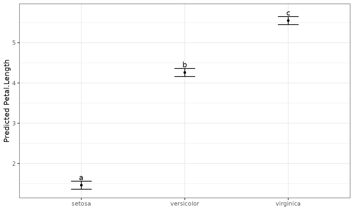
pred.out <- multiple_comparisons(model, classify = "Species")

# Display the predicted values table
pred.out
#> Multiple Comparisons of Means: Tukey's HSD Test
#> Significance level: 0.05 
#> HSD value: 0.20378 
#> 
#> Predicted values:
#>      Species predicted.value std.error  df groups   ci  low   up
#> 1     setosa            1.46      0.06 147      a 0.12 1.34 1.58
#> 2 versicolor            4.26      0.06 147      b 0.12 4.14 4.38
#> 3  virginica            5.55      0.06 147      c 0.12 5.43 5.67

# Access the p-value matrix
pred.out$pairwise_pvalues
#>                  setosa   versicolor    virginica
#> setosa     1.000000e+00 2.997602e-15 2.997602e-15
#> versicolor 2.997602e-15 1.000000e+00 2.997602e-15
#> virginica  2.997602e-15 2.997602e-15 1.000000e+00

# Access the HSD value
pred.out$hsd
#> [1] 0.20378

# Show the predicted values plot
autoplot(pred.out, label_height = 0.5)


# Use traditional confidence intervals instead of Tukey comparison intervals
pred.out.ci <- multiple_comparisons(model, classify = "Species", int.type = "ci")
pred.out.ci
#> Multiple Comparisons of Means: Tukey's HSD Test
#> Significance level: 0.05 
#> HSD value: 0.20378 
#> 
#> Predicted values:
#>      Species predicted.value std.error  df groups   ci  low   up
#> 1     setosa            1.46      0.06 147      a 0.12 1.34 1.58
#> 2 versicolor            4.26      0.06 147      b 0.12 4.14 4.38
#> 3  virginica            5.55      0.06 147      c 0.12 5.43 5.67

# Plot without confidence intervals
pred.out.none <- multiple_comparisons(model, classify = "Species", int.type = "none")
autoplot(pred.out.none)


# Use a different p-value adjustment instead of Tukey's HSD
multiple_comparisons(model, classify = "Species", adjust = "fdr")
#> Multiple Comparisons of Means: p-value adjustment = fdr 
#> Significance level: 0.05 
#> 
#> Predicted values:
#>      Species predicted.value std.error  df groups   ci  low   up
#> 1     setosa            1.46      0.06 147      a 0.12 1.34 1.58
#> 2 versicolor            4.26      0.06 147      b 0.12 4.14 4.38
#> 3  virginica            5.55      0.06 147      c 0.12 5.43 5.67

# `by`: run the comparisons independently within each level of another factor.
# Here a 2 x 3 factorial - compare tension levels within each wool type.
m_wb <- aov(breaks ~ wool * tension, data = warpbreaks)
mc_by <- multiple_comparisons(m_wb, classify = "wool:tension", by = "wool")
mc_by
#> Multiple Comparisons of Means: Tukey's HSD Test
#> Significance level: 0.05 
#> HSD value: varies by comparison (see $hsd)
#>  
#> 
#> Predicted values:
#>   wool tension predicted.value std.error df groups   ci   low    up
#> 1    A       M           24.00      3.65 48      a 7.33 16.67 31.33
#> 2    A       H           24.56      3.65 48      a 7.33 17.22 31.89
#> 3    A       L           44.56      3.65 48      b 7.33 37.22 51.89
#> 4    B       H           18.78      3.65 48      a 7.33 11.45 26.11
#> 5    B       L           28.22      3.65 48      a 7.33 20.89 35.55
#> 6    B       M           28.78      3.65 48      a 7.33 21.45 36.11
autoplot(mc_by) # faceted by wool


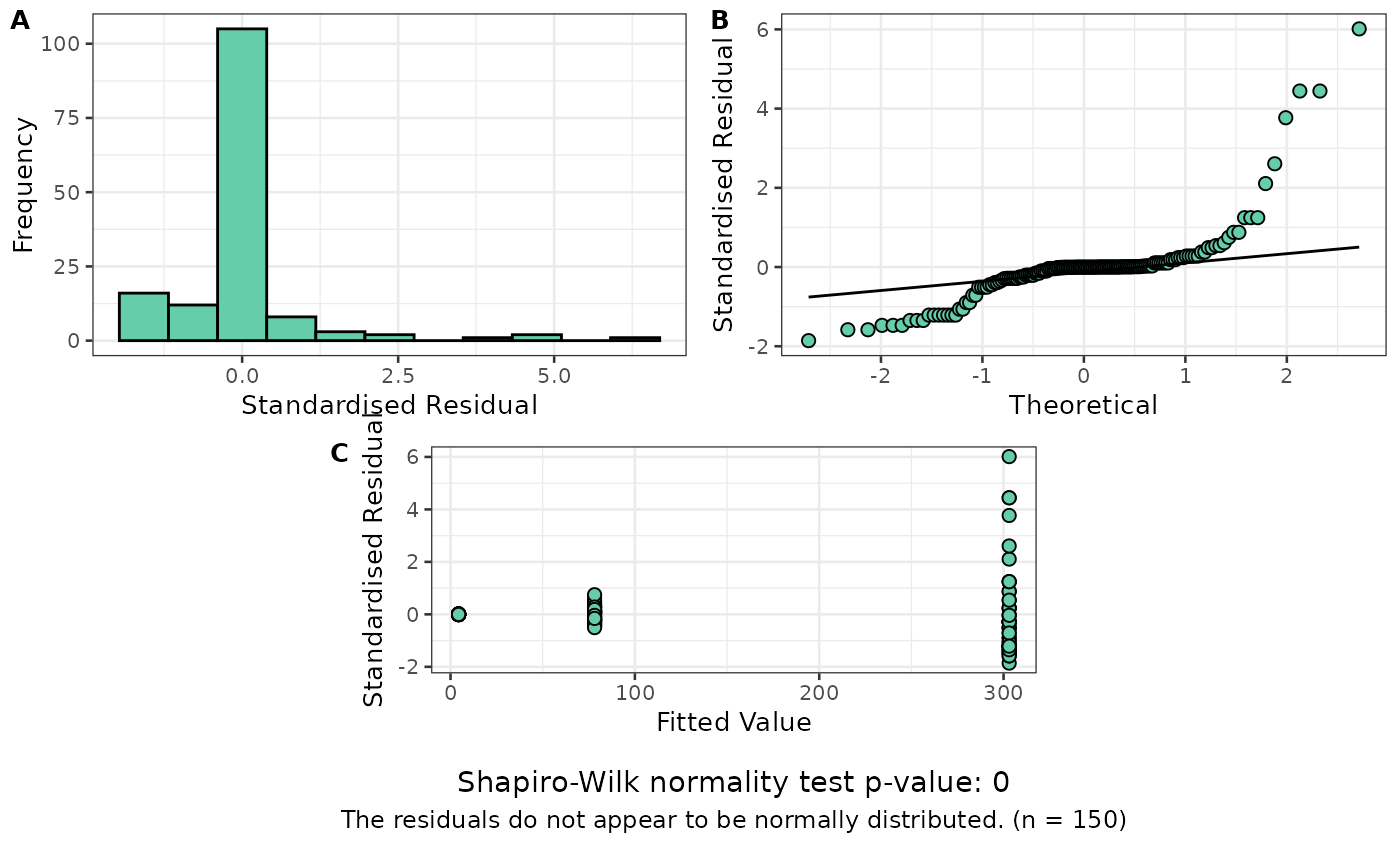
# AOV model example with transformation
my_iris <- iris
my_iris$Petal.Length <- exp(my_iris$Petal.Length) # Create exponential response
exp_model <- aov(Petal.Length ~ Species, data = my_iris)

resplot(exp_model) # Residual plot shows problems


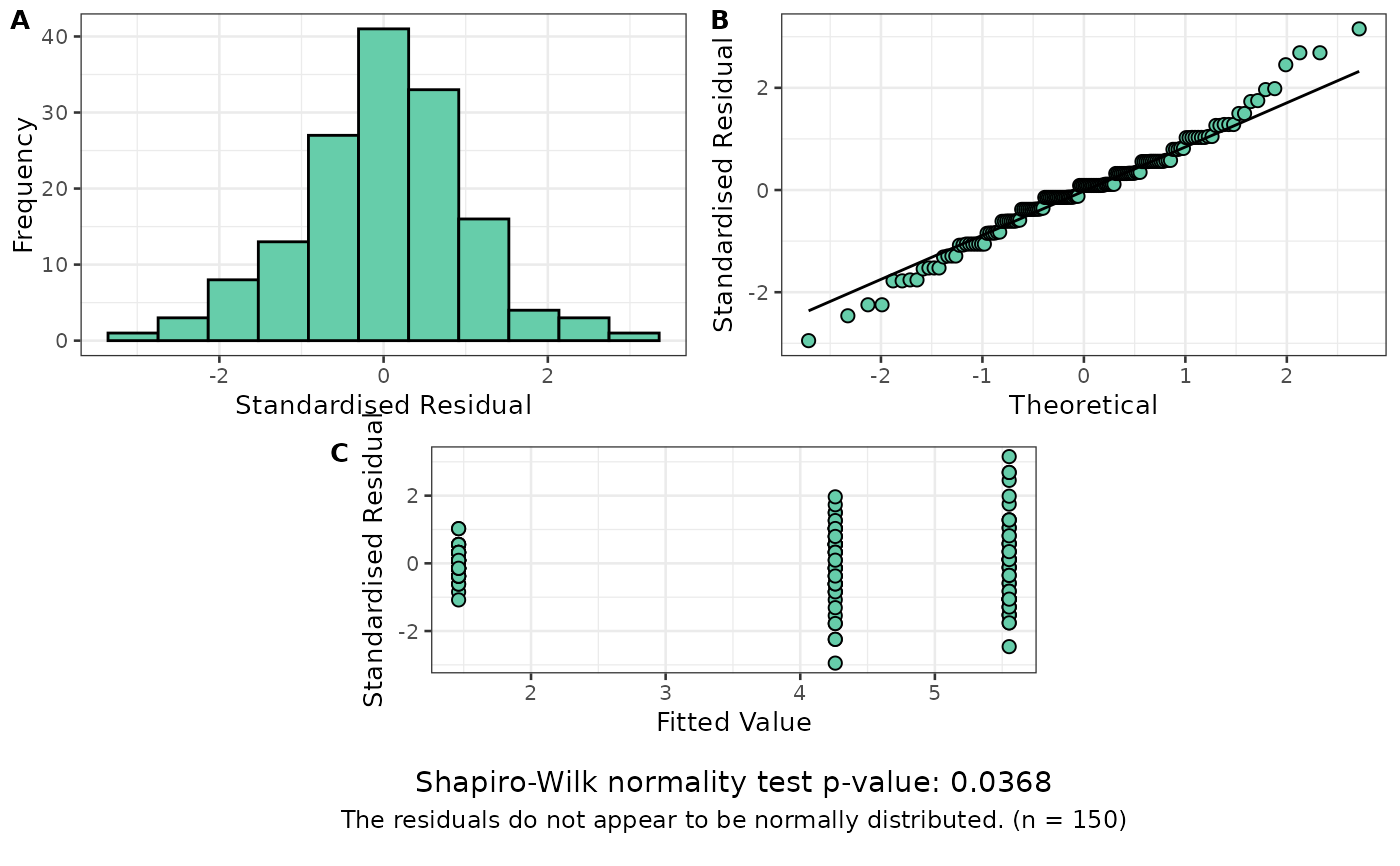
# Fit a new model using a log transformation of the response
log_model <- aov(log(Petal.Length) ~ Species, data = my_iris)

resplot(log_model) # Looks much better


# Display the ANOVA table for the model
anova(log_model)
#> Analysis of Variance Table
#> 
#> Response: log(Petal.Length)
#>            Df Sum Sq Mean Sq F value    Pr(>F)    
#> Species     2 437.10 218.551  1180.2 < 2.2e-16 ***
#> Residuals 147  27.22   0.185                      
#> ---
#> Signif. codes:  0 ‘***’ 0.001 ‘**’ 0.01 ‘*’ 0.05 ‘.’ 0.1 ‘ ’ 1

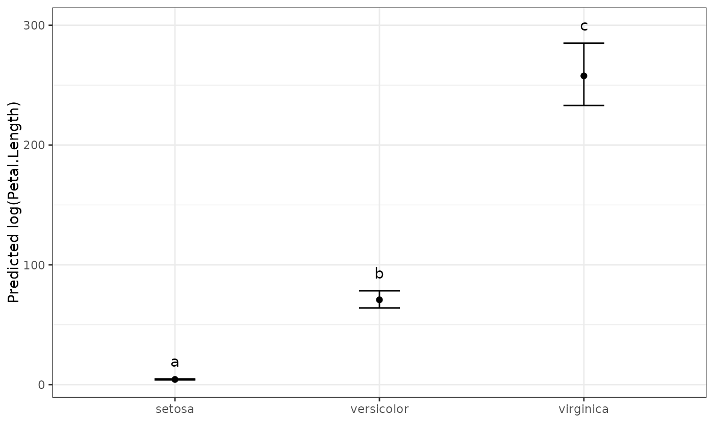
# Back transform, because the "original" data was exponential
pred.out <- multiple_comparisons(log_model, classify = "Species",
                                   trans = "log")
#> Warning: Offset value assumed to be 0. Change with `offset` argument.

# Display the predicted values table
pred.out
#> Multiple Comparisons of Means: Tukey's HSD Test
#> Significance level: 0.05 
#> HSD value: 0.20378 
#> 
#> Predicted values:
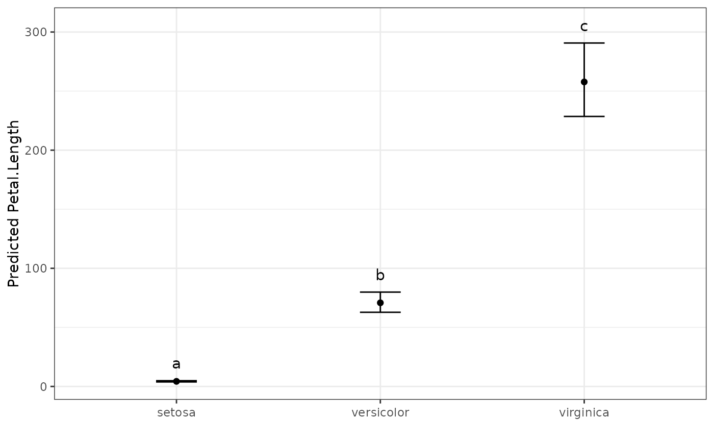
#>      Species predicted.value std.error  df groups   ci PredictedValue ApproxSE
#> 1     setosa            1.46      0.06 147      a 0.12           4.31     0.26
#> 2 versicolor            4.26      0.06 147      b 0.12          70.81     4.31
#> 3  virginica            5.55      0.06 147      c 0.12         257.75    15.69
#>      low     up
#> 1   3.83   4.87
#> 2  62.79  79.86
#> 3 228.54 290.69

# Show the predicted values plot
autoplot(pred.out, label_height = 15)


if (FALSE) { # \dontrun{
# ASReml-R Example
library(asreml)

# Fit ASReml-R model
model.asr <- asreml(yield ~ Nitrogen + Variety + Nitrogen:Variety,
                    random = ~ Blocks + Blocks:Wplots,
                    residual = ~ units,
                    data = asreml::oats)

wald(model.asr) # Nitrogen main effect significant

#Determine ranking and groups according to Tukey's Test
pred.out <- multiple_comparisons(model.obj = model.asr, classify = "Nitrogen",
                    descending = TRUE)

print(pred.out, decimals = 5)

# Example using a box-cox transformation
set.seed(42) # See the seed for reproducibility
resp <- rnorm(n = 50, 5, 1)^3
trt <- as.factor(sample(rep(LETTERS[1:10], 5), 50))
block <- as.factor(rep(1:5, each = 10))
ex_data <- data.frame(resp, trt, block)

# Change one treatment random values to get significant difference
ex_data$resp[ex_data$trt=="A"] <- rnorm(n = 5, 7, 1)^3

model.asr <- asreml(resp ~ trt,
                    random = ~ block,
                    residual = ~ units,
                    data = ex_data)

resplot(model.asr)

# lambda = 1/3 from MASS::boxcox()
model.asr <- asreml(resp^(1/3) ~ trt,
                    random = ~ block,
                    residual = ~ units,
                    data = ex_data)

resplot(model.asr) # Look much better

pred.out <- multiple_comparisons(model.obj = model.asr,
                                 classify = "trt",
                                 trans = "power", power = (1/3))

pred.out
autoplot(pred.out, label_height = 0.5)
} # }