Introduction
When presenting field trial layouts, it’s often important to provide spatial context through orientation arrows (indicating north or other directions) and annotations that reference physical features of the field (such as boundaries, gates, or adjacent landmarks). This vignette demonstrates how to add these elements to field layout plots generated by the biometryassist package.
The biometryassist package generates field layout plots as ggplot2 objects, which means we can enhance them using standard ggplot2 functions and extensions. This vignette will show you how to:
- Add orientation arrows with arbitrary rotation
- Add text annotations outside the plotting area to label field features
Setup
First, let’s load the required packages and generate a basic experimental design:
library(biometryassist)
library(ggplot2)
library(ggspatial)
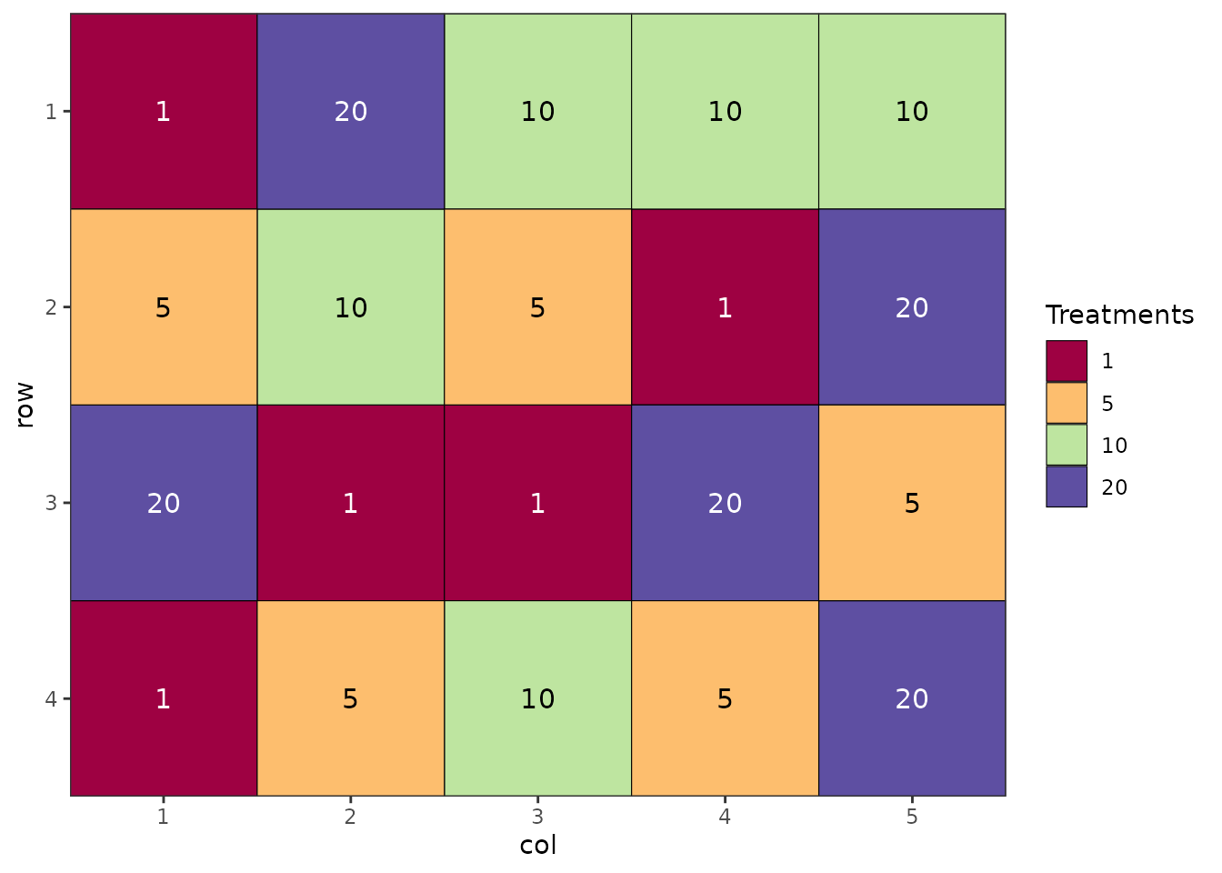
# Generate a completely randomized design (CRD)
des.out <- design(
type = "crd",
treatments = c(1, 5, 10, 20),
reps = 5,
nrows = 4,
ncols = 5,
seed = 42
)
## Source of Variation df
## =============================================
## treatments 3
## Residual 16
## =============================================
## Total 19
The design() function creates a field layout and stores it in des.out$plot.des as a ggplot2 object. We can now enhance this plot with additional annotations.
Adding an Orientation Arrow
Orientation arrows help readers understand the spatial layout of a field trial relative to cardinal directions or other reference points. This is particularly useful when field orientation affects environmental conditions like sun exposure or prevailing winds.
Using ggspatial for North Arrows
The ggspatial package provides the annotation_north_arrow() function, which is specifically designed for adding directional arrows to plots. While it’s primarily intended for spatial data with coordinate reference systems, it works well for field layout plots too.
des.out$plot.des +
  annotation_north_arrow(
    location = "tr",
    rotation = 53,
    pad_x = unit(-1.5, "cm"),
    pad_y = unit(0.5, "cm"),
    style = north_arrow_fancy_orienteering(
      line_width = 1,
      text_size = 10
    )
  ) +
  coord_cartesian(clip = "off") +
  theme(plot.margin = margin(t = 10, r = 50, b = 10, l = 10, unit = "pt"))
Let’s break down each component of this code:
annotation_north_arrow() arguments:
location = "tr": Places the arrow in the top-right corner. Other options include "tl" (top-left), "bl" (bottom-left), "br" (bottom-right), or you can specify exact coordinates as a numeric vector c(x, y).
rotation = 53: Rotates the arrow 53 degrees anti-clockwise from north. This allows you to indicate the true field orientation. For example, if north in your field is 45 degrees clockwise from the top of your plot, use rotation = 45. Use rotation = 0 if north aligns with the top of the plot.
pad_x = unit(-1.5, "cm"): Moves the arrow horizontally. Negative values move it right, positive values move it left. This allows fine-tuning of the arrow position.
pad_y = unit(0.5, "cm"): Moves the arrow vertically. Positive values move it down, negative values move it up.
-
style = north_arrow_fancy_orienteering(): Specifies the visual style of the arrow. Other available styles include:
Within each style function, you can customize:
-
line_width: Thickness of arrow lines
-
text_size: Size of the “N” label
Additional ggplot2 modifications:
coord_cartesian(clip = "off"): This is critical. By default, ggplot2 clips (cuts off) any elements that fall outside the plotting area. Setting clip = "off" allows the arrow to be drawn outside the plot panel, which is necessary when using padding to position it beyond the plot boundaries.
theme(plot.margin = ...): Expands the margins around the plot to create space for the arrow. The margin() function takes four values: top, right, bottom, left. Units are specified with the unit parameter (here, points). We increase the right margin to 50pt to accommodate the arrow.
Customizing Arrow Appearance
You can customize the arrow style parameters to match your needs:
des.out$plot.des +
  annotation_north_arrow(
    location = "tr",
    rotation = 30,  # Different rotation angle
    pad_x = unit(-1, "cm"),
    pad_y = unit(0.3, "cm"),
    style = north_arrow_minimal(  # Different style
      line_width = 1.5,
      text_size = 12
    )
  ) +
  coord_cartesian(clip = "off") +
  theme(plot.margin = margin(t = 10, r = 50, b = 10, l = 10, unit = "pt"))
Adding Field Feature Annotations
In addition to orientation, it’s often helpful to label physical features of the field site, such as boundaries, access points, or adjacent landmarks. These annotations provide practical context for field operations and help with trial management.
Using annotate() for Text Labels
The annotate() function allows us to add text (and other geometric objects) to specific locations on the plot. Unlike the north arrow, these annotations use the plot’s coordinate system.
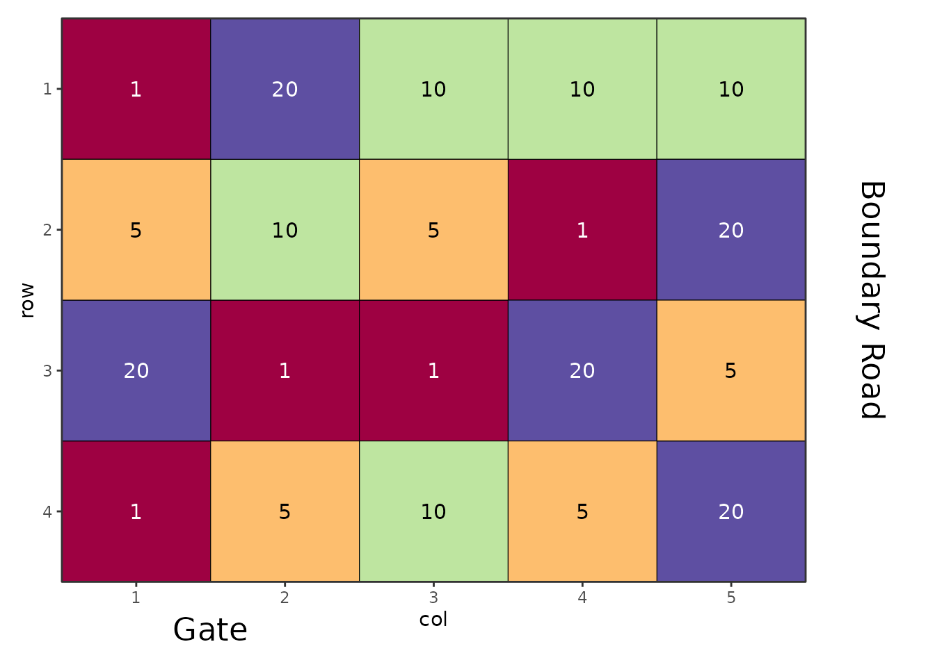
des.out$plot.des +
  annotate(
    "text",
    x = 5.8,
    y = mean(des.out$design$row),
    label = "Boundary Road",
    angle = 270,
    hjust = 0.5,
    vjust = -0.5,
    size = 6
  ) +
  annotate(
    "text",
    x = 1.5,
    y = 5,
    label = "Gate",
    hjust = 0.5,
    vjust = -0.5,
    size = 6
  ) +
  coord_cartesian(xlim = c(0.5, 5.5), ylim = c(0.5, 4.5), clip = "off") +
  theme(plot.margin = margin(t = 10, r = 70, b = 20, l = 10, unit = "pt"),
        legend.position="none")
Let’s examine each annotation in detail:
First annotation - “Boundary Road” (vertical text on right):
"text": Specifies that we’re adding a text annotation (other options include "rect", "segment", etc.)
x = 5.8: The x-coordinate for the text. Since our plot has 5 columns (numbered 1-5), placing it at 5.8 positions it outside the right edge of the plot.
y = mean(des.out$design$row): Centers the text vertically by calculating the mean of all row numbers. This ensures the text is centered regardless of the number of rows.
label = "Boundary Road": The text to display.
angle = 270: Rotates the text 270 degrees (or -90 degrees), making it read from top to bottom. This is conventional for labels on the right side of plots.
hjust = 0.5: Horizontal justification. 0.5 centers the text horizontally relative to the x-coordinate.
vjust = -0.5: Vertical justification. Negative values move the text away from the plot (outward), while positive values would move it toward the plot. This ensures the text doesn’t overlap with the plot area.
size = 6: The font size for the text.
Second annotation - “Gate” (horizontal text on top):
x = 1.5: Positions the text above column 1.5 (between columns 1 and 2).
y = 5: Places it above the top row (row 4), outside the plotting area.
angle is not specified, so the text remains horizontal (0 degrees).
Other parameters work similarly to the first annotation.
Critical settings for external annotations:
-
coord_cartesian(xlim = c(0.5, 5.5), ylim = c(0.5, 4.5), clip = "off"):
-
xlim and ylim explicitly set the visible data range. This is essential because when we add annotations with coordinates outside the data range (like x = 5.8), ggplot2 would normally expand the axis limits to include these points, stretching the plot. By explicitly setting the limits to match our original plot grid (columns 0.5-5.5, rows 0.5-4.5), we prevent this expansion.
-
clip = "off" allows drawing outside these limits, so our annotations at x = 5.8 and y = 5 are still visible.
-
theme(plot.margin = ...): Expands margins to create physical space for the text. The right margin is set to 70pt to accommodate “Boundary Road”, and the top margin is 20pt for “Gate”.
Understanding the Coordinate System
The field layout plot uses the row and column numbers as coordinates: - Columns are numbered 1 to ncols (here, 1 to 5) - Rows are numbered 1 to nrows (here, 1 to 4) - Each plot cell is centered on its integer coordinates
To position annotations: - Outside right edge: Use x > max column number (e.g., x = 5.8 when max column is 5) - Outside top edge: Use y > max row number (e.g., y = 5 when max row is 4) - Outside left edge: Use x < min column number (e.g., x = 0.2 when min column is 1) - Outside bottom edge: Use y < min row number (e.g., y = 0.2 when min row is 1)
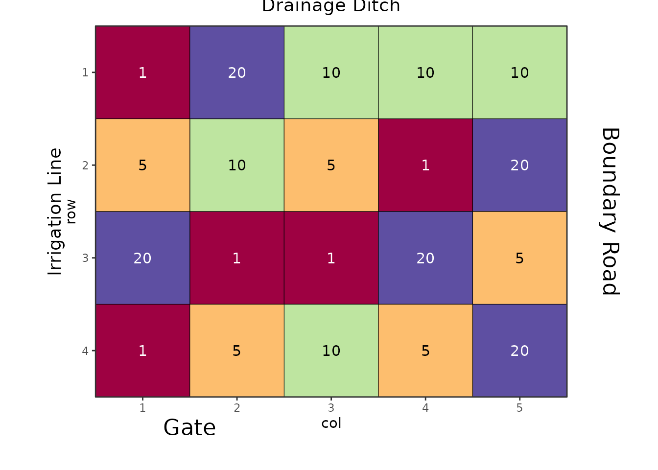
Adding Multiple Features
You can add as many annotations as needed by chaining multiple annotate() calls:
des.out$plot.des +
  annotate("text", x = 5.8, y = mean(des.out$design$row),
           label = "Boundary Road", angle = 270, hjust = 0.5, vjust = -0.5, size = 6) +
  annotate("text", x = 1.5, y = 5,
           label = "Gate", hjust = 0.5, vjust = -0.5, size = 6) +
  annotate("text", x = 0.2, y = mean(des.out$design$row),
           label = "Irrigation Line", angle = 90, hjust = 0.5, vjust = -0.5, size = 5) +
  annotate("text", x = mean(des.out$design$col), y = 0.2,
           label = "Drainage Ditch", hjust = 0.5, vjust = 1, size = 5) +
  coord_cartesian(xlim = c(0.5, 5.5), ylim = c(0.5, 4.5), clip = "off") +
  theme(plot.margin = margin(t = 20, r = 70, b = 30, l = 50, unit = "pt"),
        legend.position="none")
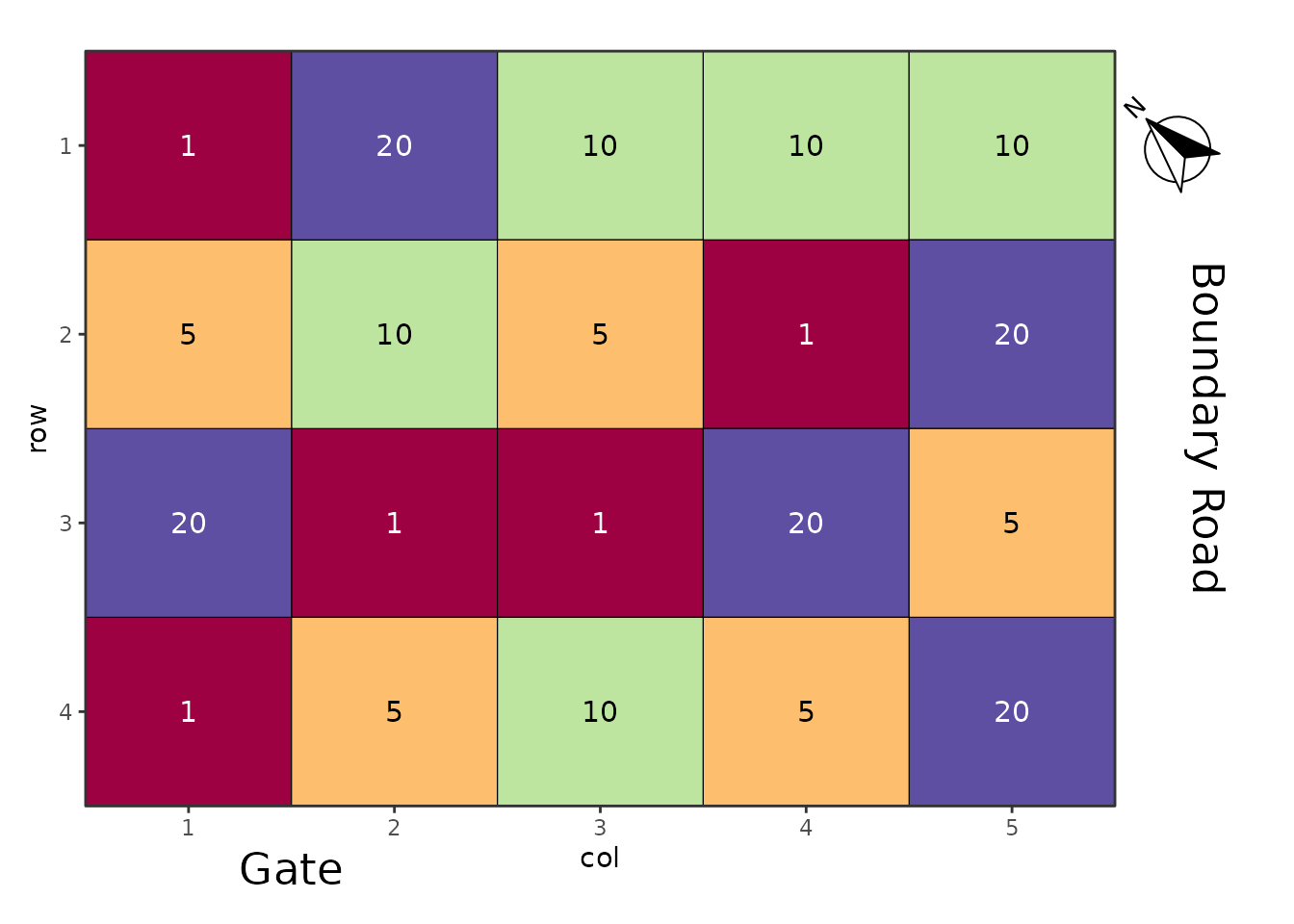
Combining Orientation Arrows and Annotations
You can combine both techniques to create a fully annotated field layout:
des.out$plot.des +
  # Add north arrow
  annotation_north_arrow(
    location = "tr",
    rotation = 45,
    pad_x = unit(-1.5, "cm"),
    pad_y = unit(0.5, "cm"),
    style = north_arrow_fancy_orienteering(line_width = 1, text_size = 10)
  ) +
  # Add field feature annotations
  annotate("text", x = 5.8, y = mean(des.out$design$row),
           label = "Boundary Road", angle = 270, hjust = 0.5, vjust = -0.5, size = 6) +
  annotate("text", x = 1.5, y = 5,
           label = "Gate", hjust = 0.5, vjust = -0.5, size = 6) +
  # Apply coordinate system and theme adjustments
  coord_cartesian(xlim = c(0.5, 5.5), ylim = c(0.5, 4.5), clip = "off") +
  theme(plot.margin = margin(t = 20, r = 70, b = 20, l = 10, unit = "pt"),
        legend.position="none")
Tips and Best Practices
Determining Appropriate Coordinates
To find the right coordinates for your annotations:
-
Check the design dimensions: Use
str(des.out$design) to see the row and column ranges
-
Use summary functions:
mean(), min(), and max() help center or position annotations
-
Experiment iteratively: Start with approximate values and adjust based on the output
Adjusting Margins
If your annotations are cut off or too far from the plot:
-
Increase margin if text is cut off:
margin(t = 30, r = 80, ...)
-
Decrease margin if there’s too much white space:
margin(t = 10, r = 40, ...)
- Margins are specified as: top, right, bottom, left
Text Rotation Guidelines
-
angle = 0: Horizontal text (default)
-
angle = 90: Vertical text, reading bottom-to-top
-
angle = 270 or angle = -90: Vertical text, reading top-to-bottom (conventional for right-side labels)
-
angle = 45: Diagonal text (sometimes useful for corner annotations)
Justification Parameters
-
hjust = 0: Left-aligned
-
hjust = 0.5: Center-aligned (most common)
-
hjust = 1: Right-aligned
-
vjust = 0: Bottom-aligned
-
vjust = 0.5: Middle-aligned
-
vjust = 1: Top-aligned
For external annotations, vjust values outside 0-1 (like vjust = -0.5) create spacing between the text and the plot edge.
Working with Different Design Types
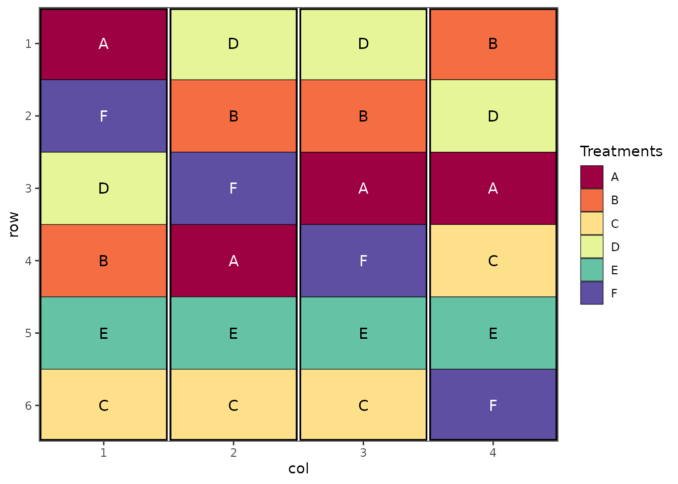
These techniques work with any design type generated by biometryassist. Here’s an example with a randomized complete block design (RCBD):
# Generate an RCBD
des.rcbd <- design(
  type = "rcbd",
  treatments = LETTERS[1:6],
  reps = 4,
  nrows = 6,
  ncols = 4,
  brows = 6,
  bcols = 1,
  seed = 123
)
## Source of Variation                     df
## =============================================
## Block stratum                           3
## ---------------------------------------------
## treatments                              5
## Residual                                15
## =============================================
## Total                                   23
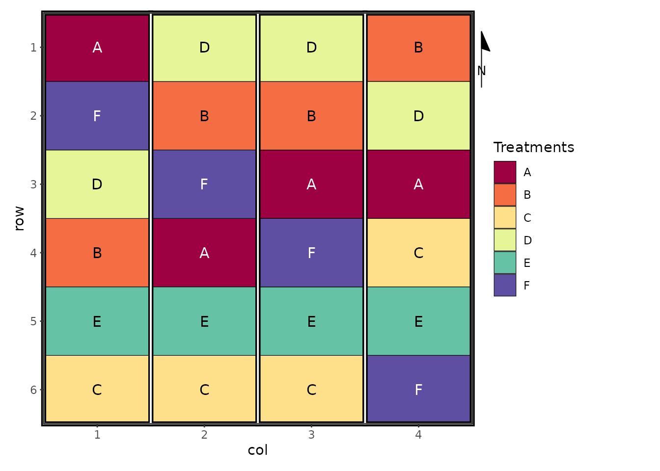
# Add annotations
des.rcbd$plot.des +
  annotation_north_arrow(
    location = "tr",
    rotation = 0,
    pad_x = unit(-1, "cm"),
    pad_y = unit(0.5, "cm"),
    style = north_arrow_minimal(line_width = 1, text_size = 10)
  ) +
  annotate("text", x = 4.8, y = mean(des.rcbd$design$row),
           label = "Access Road", angle = 270, hjust = 0.5, vjust = -0.5, size = 5) +
  coord_cartesian(xlim = c(0.5, 4.5), ylim = c(0.5, 6.5), clip = "off") +
  theme(plot.margin = margin(t = 10, r = 60, b = 10, l = 10, unit = "pt"))
Note how the coordinate limits (xlim and ylim) are adjusted to match the dimensions of this design (4 columns, 6 rows).
Troubleshooting
Problem: Annotation is cut off
Solution: Increase the relevant plot margin using theme(plot.margin = margin(...)). Ensure margins are large enough to accommodate your text.
Problem: Plot is stretched or distorted
Solution: When using annotate() with coordinates outside the plot range, always specify explicit limits in coord_cartesian(xlim = ..., ylim = ...) to prevent automatic axis expansion.
Problem: North arrow is not visible
Solution: 1. Check that coord_cartesian(clip = "off") is included 2. Verify that plot margins are large enough 3. Adjust pad_x and pad_y values to position the arrow within the margin area
Problem: Text orientation is wrong
Solution: Adjust the angle parameter: - For right side labels reading upward: angle = 90 - For right side labels reading downward (conventional): angle = 270 - For left side labels: reverse these angles
Conclusion
Adding orientation arrows and field feature annotations to your experimental design plots enhances their utility for field management, reporting, and publication. The combination of ggspatial::annotation_north_arrow() for directional reference and ggplot2::annotate() for custom labels provides flexible tools for creating publication-ready field layout diagrams.
Remember the key principles: - Use coord_cartesian(clip = "off") to allow drawing outside the plot panel - Set appropriate plot.margin values to create space for external elements - For annotate(), explicitly set xlim and ylim to prevent axis stretching - Experiment with positioning and adjust iteratively