Produces a plot of the plot/field layout for a design() result, with plots
coloured by treatment and block boundaries drawn for blocked designs.
Usage
# S3 method for class 'design'
autoplot(
  object,
  rotation = 0,
  size = 4,
  margin = FALSE,
  palette = "default",
  row = NULL,
  column = NULL,
  block = NULL,
  treatments = NULL,
  legend = TRUE,
  ...
)
Arguments
- object
A
designobject, as produced bydesign().- rotation
Rotate the treatment labels within the plot. Allows for easier reading of long treatment labels. Number between 0 and 360 (inclusive) - default 0
- size
Increase or decrease the text size within the plot for treatment labels. Numeric with default value of 4.
- margin
Logical (default
FALSE). A value ofFALSEwill expand the plot to the edges of the plotting area i.e. remove white space between plot and axes.- palette
A string specifying the colour scheme to use for plotting or a vector of custom colours to use as the palette. Default is equivalent to "Spectral". Colour blind friendly palettes can also be provided via options
"colour blind"(or"colour blind", both equivalent to"viridis"),"magma","inferno","plasma","cividis","rocket","mako"or"turbo". Other palettes fromscales::brewer_pal()are also possible.- row
A variable to plot a column from
objectas rows.- column
A variable to plot a column from
objectas columns.- block
A variable to plot a column from
objectas blocks.- treatments
A variable to plot a column from
objectas treatments.- legend
Logical (default
TRUE). IfTRUE, displays the legend for treatment colours.- ...
Arguments passed to
ggplot2::geom_text()for the plot labels.
Examples
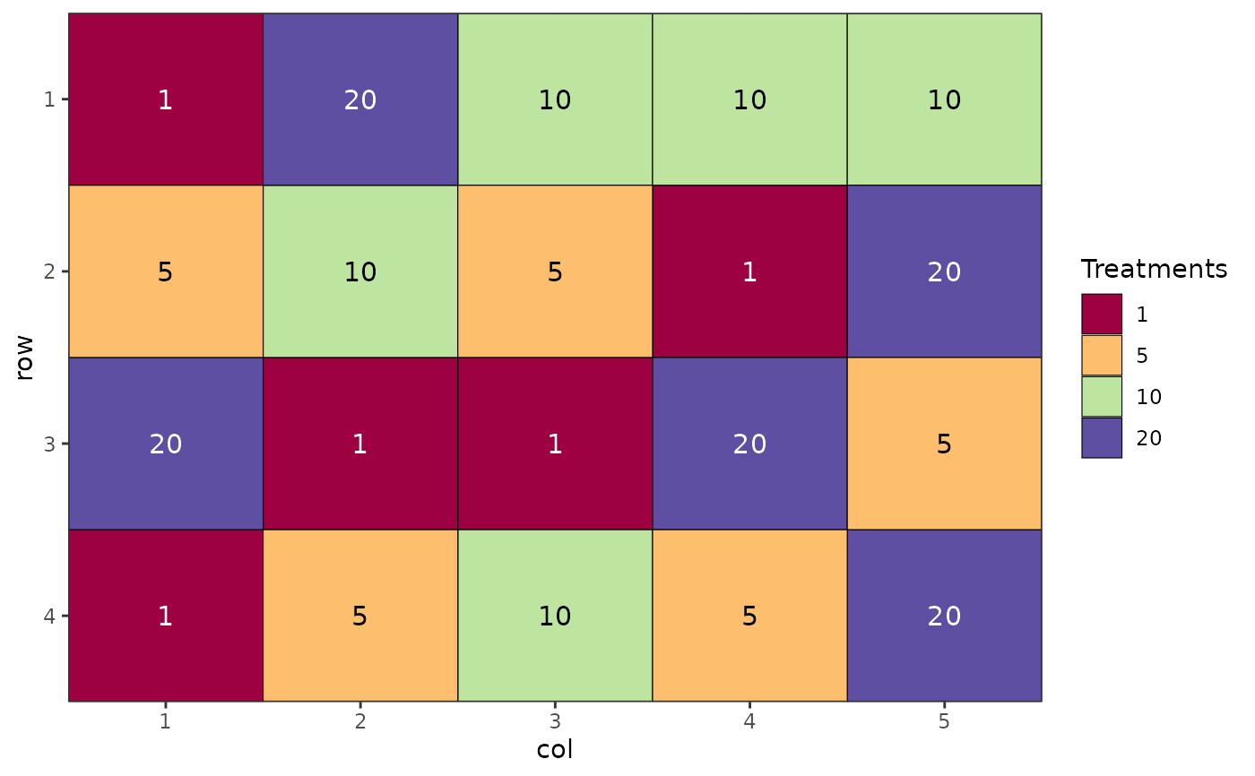
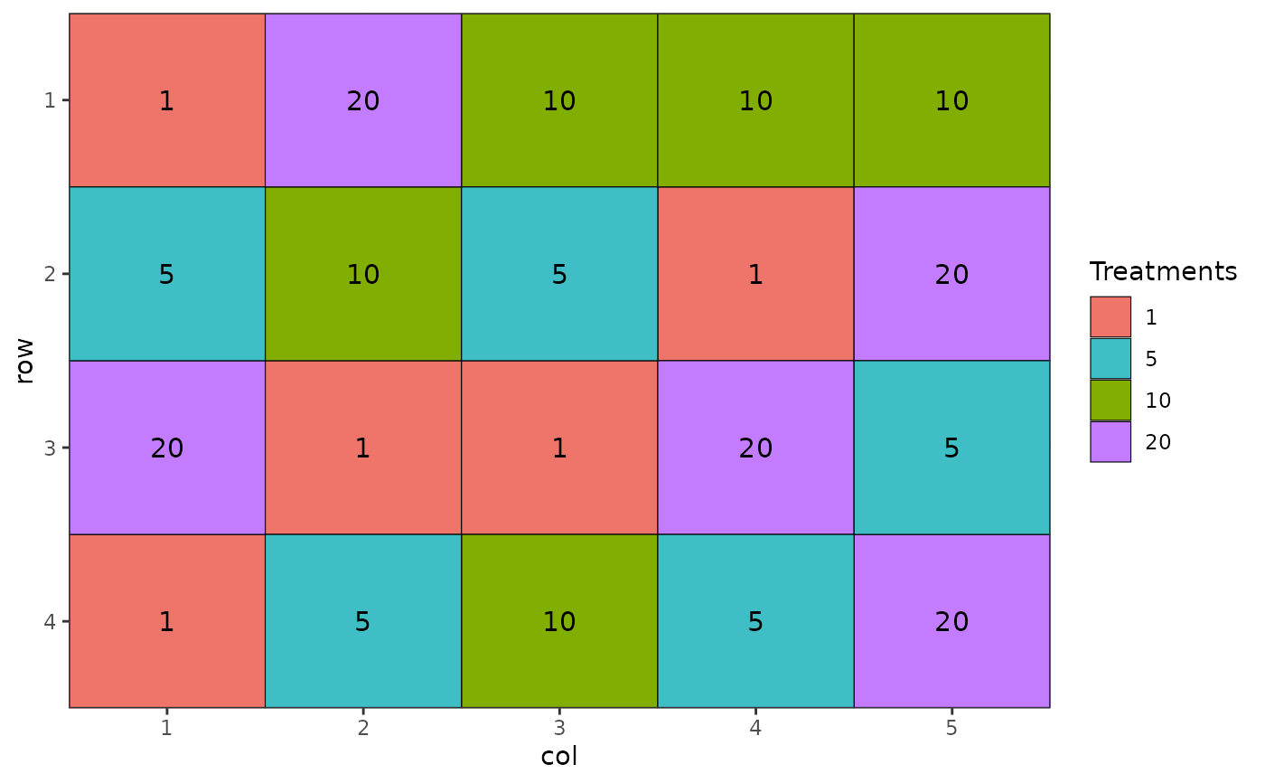
des.out <- design(type = "crd", treatments = c(1, 5, 10, 20),
reps = 5, nrows = 4, ncols = 5, seed = 42, plot = FALSE)
#> Source of Variation df
#> =============================================
#> treatments 3
#> Residual 16
#> =============================================
#> Total 19
autoplot(des.out)
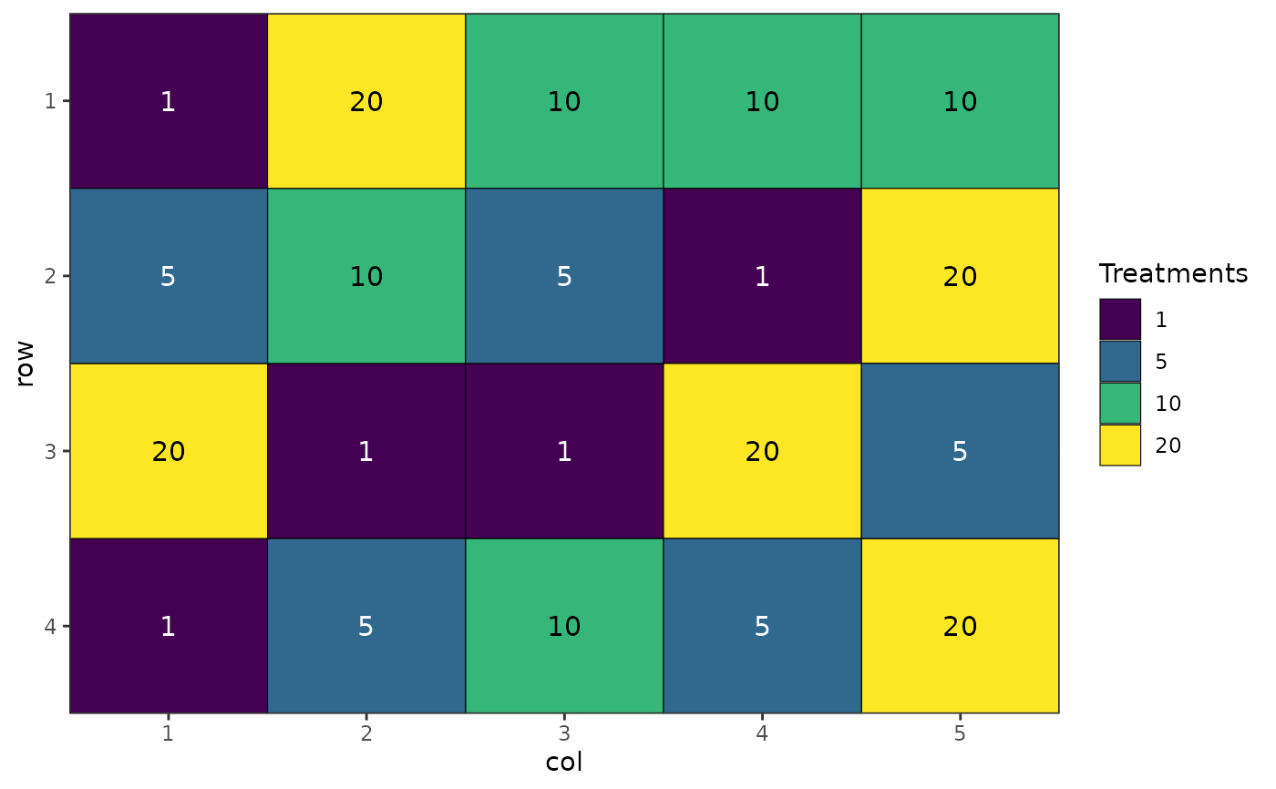
 # Colour blind friendly colours
autoplot(des.out, palette = "colour-blind")
# Colour blind friendly colours
autoplot(des.out, palette = "colour-blind")
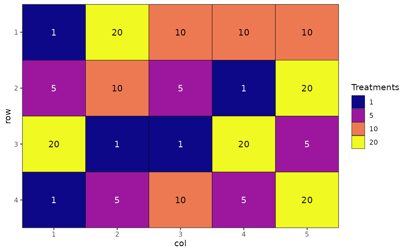
 # Alternative colour scheme
autoplot(des.out, palette = "plasma")
# Alternative colour scheme
autoplot(des.out, palette = "plasma")
 # Custom colour palette
autoplot(des.out, palette = c("#ef746a", "#3fbfc5", "#81ae00", "#c37cff"))
# Custom colour palette
autoplot(des.out, palette = c("#ef746a", "#3fbfc5", "#81ae00", "#c37cff"))
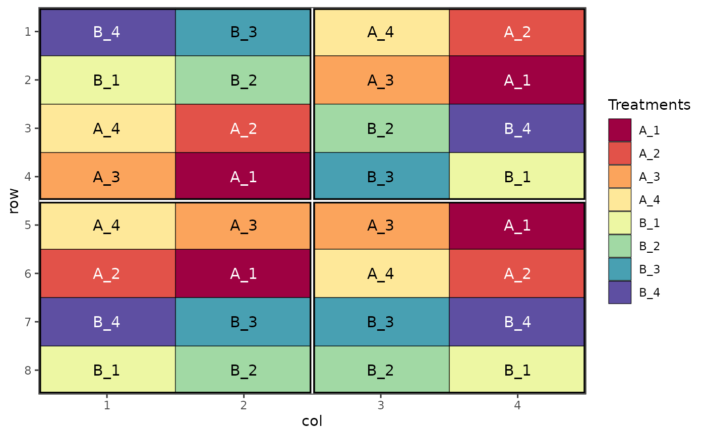
 # Visualise different components of a split plot design
des.out <- design(type = "split", treatments = c("A", "B"), sub_treatments = 1:4,
reps = 4, nrows = 8, ncols = 4, brows = 4, bcols = 2, seed = 42)
#> Source of Variation df
#> ==================================================
#> Block stratum 3
#> --------------------------------------------------
#> Whole plot stratum
#> treatments 1
#> Whole plot Residual 3
#> ==================================================
#> Subplot stratum
#> sub_treatments 3
#> treatments:sub_treatments 3
#> Subplot Residual 18
#> ==================================================
#> Total 31
# Visualise different components of a split plot design
des.out <- design(type = "split", treatments = c("A", "B"), sub_treatments = 1:4,
reps = 4, nrows = 8, ncols = 4, brows = 4, bcols = 2, seed = 42)
#> Source of Variation df
#> ==================================================
#> Block stratum 3
#> --------------------------------------------------
#> Whole plot stratum
#> treatments 1
#> Whole plot Residual 3
#> ==================================================
#> Subplot stratum
#> sub_treatments 3
#> treatments:sub_treatments 3
#> Subplot Residual 18
#> ==================================================
#> Total 31
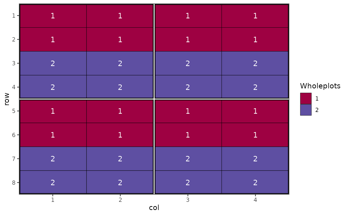
 # Show the wholeplot components
autoplot(des.out, treatments = wholeplots)
# Show the wholeplot components
autoplot(des.out, treatments = wholeplots)
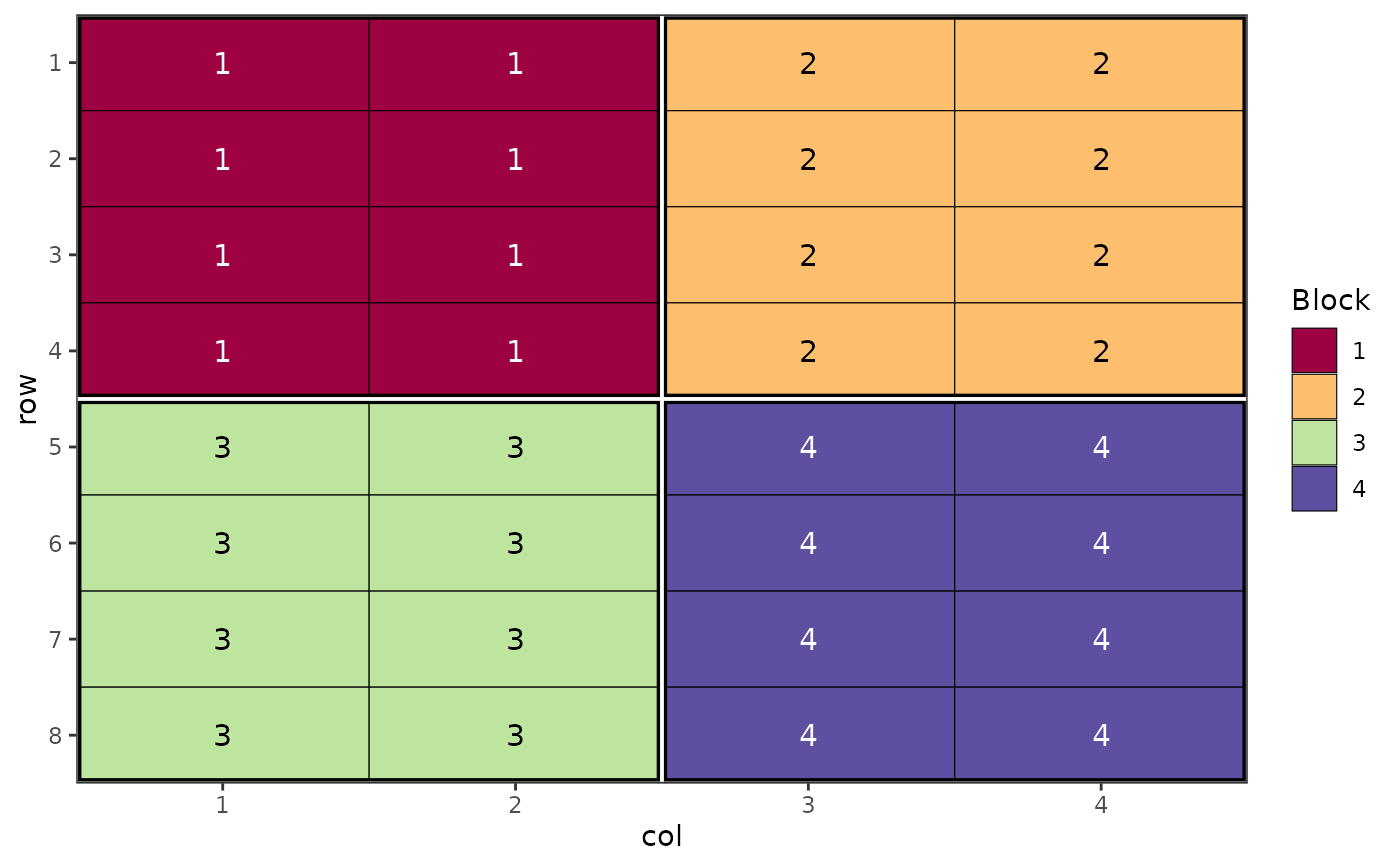
 # Display block level
autoplot(des.out, treatments = block)
# Display block level
autoplot(des.out, treatments = block)