Create a complete experimental design with graph of design layout and skeletal ANOVA table
Source:R/design.R
design.RdCreate a complete experimental design with graph of design layout and skeletal ANOVA table
Usage
design(
  type,
  treatments,
  reps,
  nrows,
  ncols,
  brows = NA,
  bcols = NA,
  byrow = TRUE,
  sub_treatments = NULL,
  fac.names = NULL,
  fac.sep = c("", " "),
  buffer = NULL,
  plot_numbers = FALSE,
  plot = TRUE,
  rotation = 0,
  size = 4,
  margin = FALSE,
  save = FALSE,
  savename = paste0(type, "_design"),
  plottype = "pdf",
  seed = TRUE,
  quiet = FALSE,
  ...
)
Arguments
- type
The design type. One of
crd,rcbd,lsd,split,strip, or a crossed factorial specified ascrossed:<base>where<base>is one ofcrd,rcbd, orlsd.- treatments
A vector containing the treatment names or labels. For split-plot designs, these treatments are applied to whole-plots. For strip-plot designs, these treatments are applied to row-strips (entire rows within each block receive the same treatment).
- reps
The number of replicates. Ignored for Latin Square Designs.
- nrows
The number of rows in the design.
- ncols
The number of columns in the design.
- brows
For RCBD, split-plot and strip-plot designs. The number of rows in a block.
- bcols
For RCBD, split-plot and strip-plot designs. The number of columns in a block.
- byrow
For split-plot and strip-plot designs. Logical (default
TRUE). Controls the within-block arrangement when there are multiple valid layouts.- sub_treatments
A vector of treatments for the sub-plot factor (required for
splitandstrip). For strip-plot designs, these treatments are applied to column-strips (entire columns within each block receive the same treatment). To apply treatments to columns instead of rows, swap thetreatmentsandsub_treatmentsarguments.- fac.names
Allows renaming of the
Alevel of factorial designs by passing (optionally named) vectors of new labels to be applied to the factors within a list. See examples and details for more information.- fac.sep
The separator used by
fac.names. Used to combine factorial design levels. If a vector of 2 levels is supplied, the first separates factor levels and label, and the second separates the different factors.- buffer
A string specifying the buffer plots to include for plotting. Default is
NULL(no buffers plotted). Other options are "edge" (outer edge of trial area), "rows" (between rows), "columns" (between columns), "double row" (a buffer row each side of a treatment row), "double column" (a buffer row each side of a treatment column), "blocks" (buffers at internal boundaries between adjacent blocks), or "double block"/"entire block"/"full block" (buffers fully surrounding each block).- plot_numbers
One of
FALSE(default),TRUE/"sequential", or"serpentine". Controls whether aplot_numbercolumn is added to the design."sequential"(orTRUE) numbers plots row-by-row from top-left to bottom-right;"serpentine"reverses direction on alternate rows, following typical field navigation paths. Plot numbers are assigned after any buffers are added, so buffer plots are numbered alongside treatment plots.- plot
Logical (default
TRUE). IfTRUE, display a plot of the generated design. A plot can always be produced later usingautoplot().- rotation
Rotate the text output as Treatments within the plot. Allows for easier reading of long treatment labels. Takes positive and negative values being number of degrees of rotation from horizontal.
- size
Increase or decrease the text size within the plot for treatment labels. Numeric with default value of 4.
- margin
Logical (default
FALSE). Expand the plot to the edges of the plotting area i.e. remove white space between plot and axes.- save
One of
FALSE(default)/"none",TRUE/"both","plot"or"workbook". Specifies which output to save.- savename
A file name for the design to be saved to. Default is the type of the design combined with "_design".
- plottype
The type of file to save the plot as. Usually one of
"pdf","png", or"jpg". Seeggplot2::ggsave()for all possible options.- seed
Logical (default
TRUE). IfTRUE, return the seed used to generate the design. If a numeric value, use that value as the seed for the design.- quiet
Logical (default
FALSE). Hide the output.- ...
Additional parameters passed to
ggplot2::ggsave()for saving the plot.
Value
A list containing a data frame with the complete design ($design), a ggplot object with plot layout ($plot.des), the seed ($seed, if return.seed = TRUE), and the satab object ($satab), allowing repeat output of the satab table via cat(output$satab).
Details
Supported designs are Completely Randomised (crd), Randomised Complete Block (rcbd), Latin Square (lsd), split-plot (split), strip-plot (strip), and crossed factorial designs via crossed:<base> where <base> is crd, rcbd, or lsd (e.g. crossed:crd).
If save = TRUE (or "both"), both the plot and the workbook will be saved to the current working directory, with filename given by savename. If one of either "plot" or "workbook" is specified, only that output is saved. If save = FALSE (the default, or equivalently "none"), nothing will be output.
fac.names can be supplied to provide more intuitive names for factors and their levels in factorial and split plot designs. They can be specified in a list format, for example fac.names = list(A_names = c("a", "b", "c"), B_names = c("x", "y", "z")). This will result a design output with a column named A_names with levels a, b, c and another named B_names with levels x, y, z. Labels can also be supplied as a character vector (e.g. c("A", "B")) which will result in only the treatment column names being renamed. Only the first two elements of the list will be used, except in the case of a 3-way factorial design.
... allows extra arguments to be passed to ggsave() for output of the plot. The details of possible arguments can be found in ggplot2::ggsave().
Examples
# Completely Randomised Design
des.out <- design(type = "crd", treatments = c(1, 5, 10, 20),
reps = 5, nrows = 4, ncols = 5, seed = 42)
#> Source of Variation df
#> =============================================
#> treatments 3
#> Residual 16
#> =============================================
#> Total 19
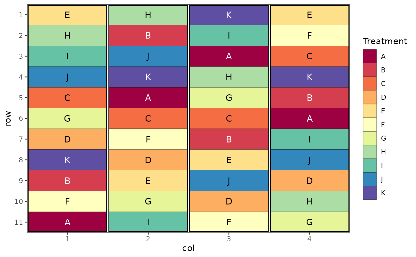
 # Randomised Complete Block Design
des.out <- design("rcbd", treatments = LETTERS[1:11], reps = 4,
nrows = 11, ncols = 4, brows = 11, bcols = 1, seed = 42)
#> Source of Variation df
#> =============================================
#> Block stratum 3
#> ---------------------------------------------
#> treatments 10
#> Residual 30
#> =============================================
#> Total 43
# Randomised Complete Block Design
des.out <- design("rcbd", treatments = LETTERS[1:11], reps = 4,
nrows = 11, ncols = 4, brows = 11, bcols = 1, seed = 42)
#> Source of Variation df
#> =============================================
#> Block stratum 3
#> ---------------------------------------------
#> treatments 10
#> Residual 30
#> =============================================
#> Total 43
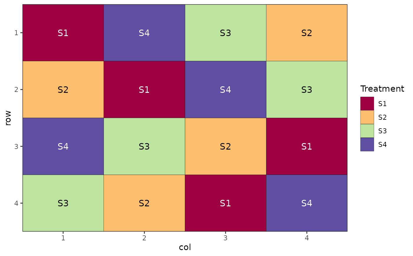
 # Latin Square Design
# Doesn't require reps argument
des.out <- design(type = "lsd", c("S1", "S2", "S3", "S4"),
nrows = 4, ncols = 4, seed = 42)
#> Source of Variation df
#> =============================================
#> Row 3
#> Column 3
#> treatments 3
#> Residual 6
#> =============================================
#> Total 15
# Latin Square Design
# Doesn't require reps argument
des.out <- design(type = "lsd", c("S1", "S2", "S3", "S4"),
nrows = 4, ncols = 4, seed = 42)
#> Source of Variation df
#> =============================================
#> Row 3
#> Column 3
#> treatments 3
#> Residual 6
#> =============================================
#> Total 15
 # Factorial Design (Crossed, Completely Randomised)
des.out <- design(type = "crossed:crd", treatments = c(3, 2),
reps = 3, nrows = 6, ncols = 3, seed = 42)
#> Source of Variation df
#> =============================================
#> A 2
#> B 1
#> A:B 2
#> Residual 12
#> =============================================
#> Total 17
# Factorial Design (Crossed, Completely Randomised)
des.out <- design(type = "crossed:crd", treatments = c(3, 2),
reps = 3, nrows = 6, ncols = 3, seed = 42)
#> Source of Variation df
#> =============================================
#> A 2
#> B 1
#> A:B 2
#> Residual 12
#> =============================================
#> Total 17
 # Factorial Design (Crossed, Completely Randomised), renaming factors
des.out <- design(type = "crossed:crd", treatments = c(3, 2),
reps = 3, nrows = 6, ncols = 3, seed = 42,
fac.names = list(N = c(50, 100, 150),
Water = c("Irrigated", "Rain-fed")))
#> Source of Variation df
#> =============================================
#> N 2
#> Water 1
#> N:Water 2
#> Residual 12
#> =============================================
#> Total 17
# Factorial Design (Crossed, Completely Randomised), renaming factors
des.out <- design(type = "crossed:crd", treatments = c(3, 2),
reps = 3, nrows = 6, ncols = 3, seed = 42,
fac.names = list(N = c(50, 100, 150),
Water = c("Irrigated", "Rain-fed")))
#> Source of Variation df
#> =============================================
#> N 2
#> Water 1
#> N:Water 2
#> Residual 12
#> =============================================
#> Total 17
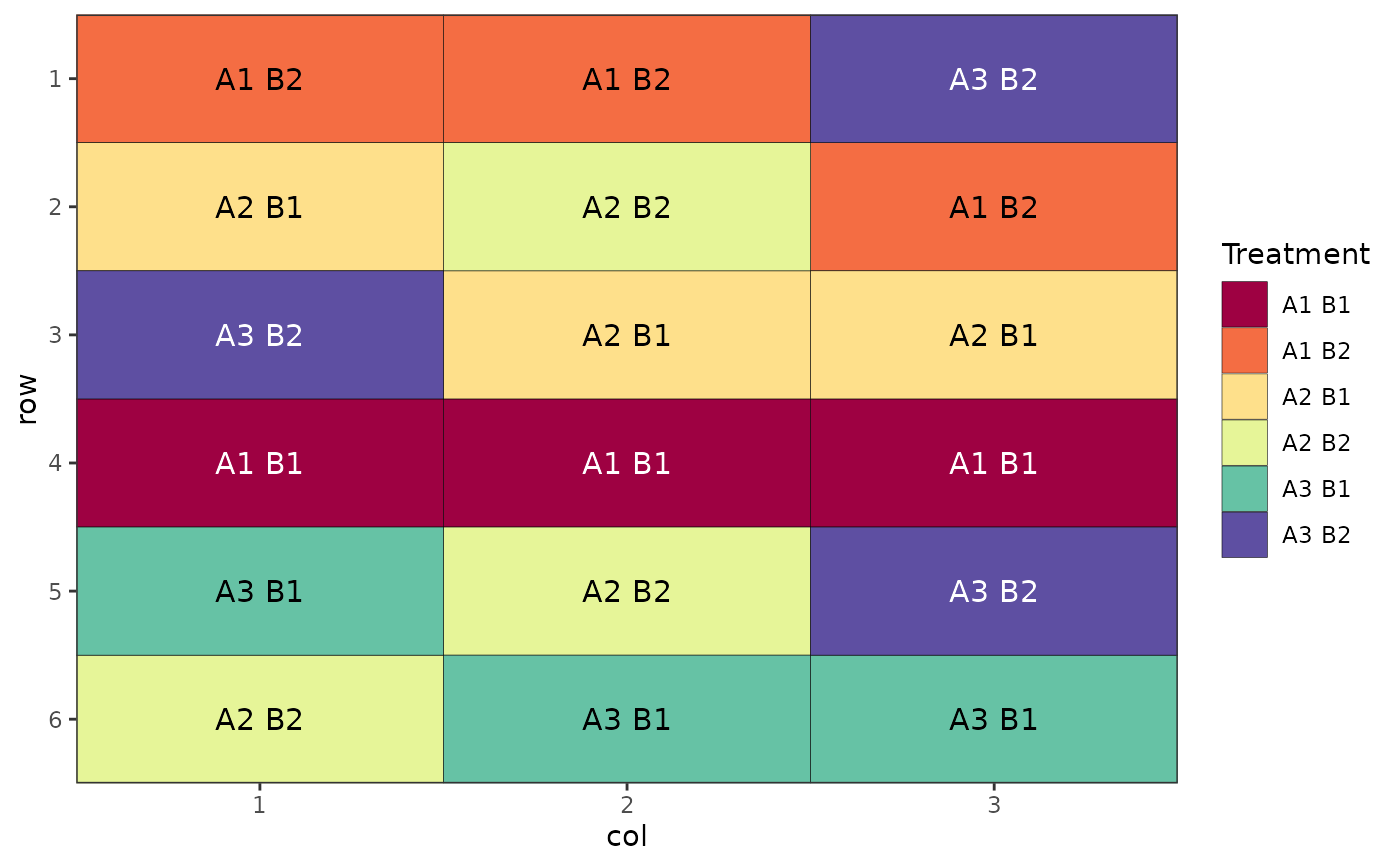
 # Factorial Design (Crossed, Randomised Complete Block Design),
# changing separation between factors
des.out <- design(type = "crossed:rcbd", treatments = c(3, 2),
reps = 3, nrows = 6, ncols = 3,
brows = 6, bcols = 1,
seed = 42, fac.sep = c(":", "_"))
#> Source of Variation df
#> =============================================
#> Block stratum 2
#> ---------------------------------------------
#> A 2
#> B 1
#> A:B 2
#> Residual 10
#> =============================================
#> Total 17
# Factorial Design (Crossed, Randomised Complete Block Design),
# changing separation between factors
des.out <- design(type = "crossed:rcbd", treatments = c(3, 2),
reps = 3, nrows = 6, ncols = 3,
brows = 6, bcols = 1,
seed = 42, fac.sep = c(":", "_"))
#> Source of Variation df
#> =============================================
#> Block stratum 2
#> ---------------------------------------------
#> A 2
#> B 1
#> A:B 2
#> Residual 10
#> =============================================
#> Total 17
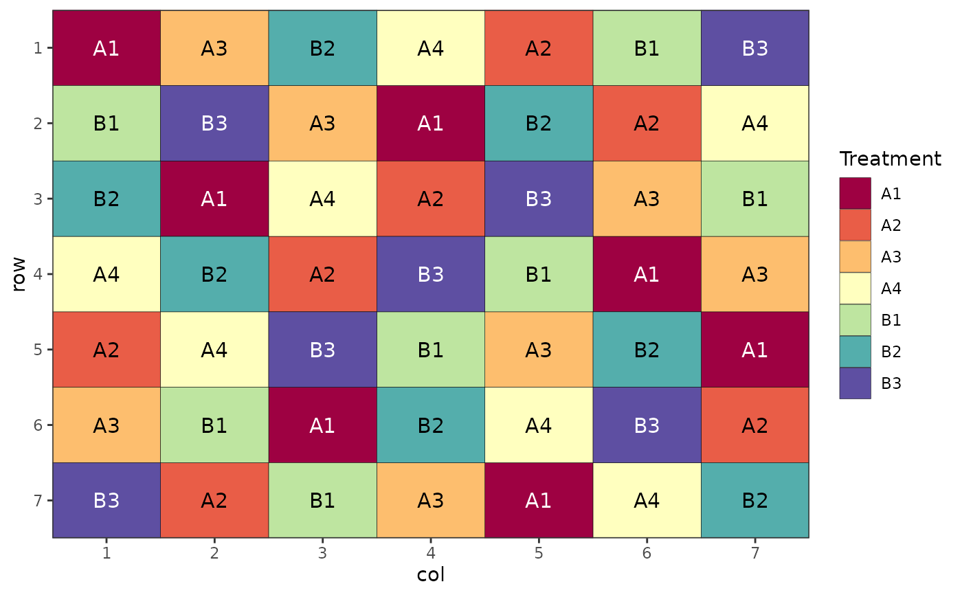
 # Factorial Design (Nested, Latin Square)
trt <- c("A1", "A2", "A3", "A4", "B1", "B2", "B3")
des.out <- design(type = "lsd", treatments = trt,
nrows = 7, ncols = 7, seed = 42)
#> Source of Variation df
#> =============================================
#> Row 6
#> Column 6
#> treatments 6
#> Residual 30
#> =============================================
#> Total 48
# Factorial Design (Nested, Latin Square)
trt <- c("A1", "A2", "A3", "A4", "B1", "B2", "B3")
des.out <- design(type = "lsd", treatments = trt,
nrows = 7, ncols = 7, seed = 42)
#> Source of Variation df
#> =============================================
#> Row 6
#> Column 6
#> treatments 6
#> Residual 30
#> =============================================
#> Total 48
 # Split plot design
des.out <- design(type = "split", treatments = c("A", "B"), sub_treatments = 1:4,
reps = 4, nrows = 8, ncols = 4, brows = 4, bcols = 2, seed = 42)
#> Source of Variation df
#> ==================================================
#> Block stratum 3
#> --------------------------------------------------
#> Whole plot stratum
#> treatments 1
#> Whole plot Residual 3
#> ==================================================
#> Subplot stratum
#> sub_treatments 3
#> treatments:sub_treatments 3
#> Subplot Residual 18
#> ==================================================
#> Total 31
# Split plot design
des.out <- design(type = "split", treatments = c("A", "B"), sub_treatments = 1:4,
reps = 4, nrows = 8, ncols = 4, brows = 4, bcols = 2, seed = 42)
#> Source of Variation df
#> ==================================================
#> Block stratum 3
#> --------------------------------------------------
#> Whole plot stratum
#> treatments 1
#> Whole plot Residual 3
#> ==================================================
#> Subplot stratum
#> sub_treatments 3
#> treatments:sub_treatments 3
#> Subplot Residual 18
#> ==================================================
#> Total 31
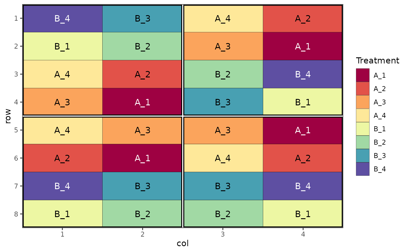 # Alternative arrangement of the same design as above
des.out <- design(type = "split", treatments = c("A", "B"), sub_treatments = 1:4,
reps = 4, nrows = 8, ncols = 4, brows = 4, bcols = 2,
byrow = FALSE, seed = 42)
#> Source of Variation df
#> ==================================================
#> Block stratum 3
#> --------------------------------------------------
#> Whole plot stratum
#> treatments 1
#> Whole plot Residual 3
#> ==================================================
#> Subplot stratum
#> sub_treatments 3
#> treatments:sub_treatments 3
#> Subplot Residual 18
#> ==================================================
#> Total 31
# Alternative arrangement of the same design as above
des.out <- design(type = "split", treatments = c("A", "B"), sub_treatments = 1:4,
reps = 4, nrows = 8, ncols = 4, brows = 4, bcols = 2,
byrow = FALSE, seed = 42)
#> Source of Variation df
#> ==================================================
#> Block stratum 3
#> --------------------------------------------------
#> Whole plot stratum
#> treatments 1
#> Whole plot Residual 3
#> ==================================================
#> Subplot stratum
#> sub_treatments 3
#> treatments:sub_treatments 3
#> Subplot Residual 18
#> ==================================================
#> Total 31
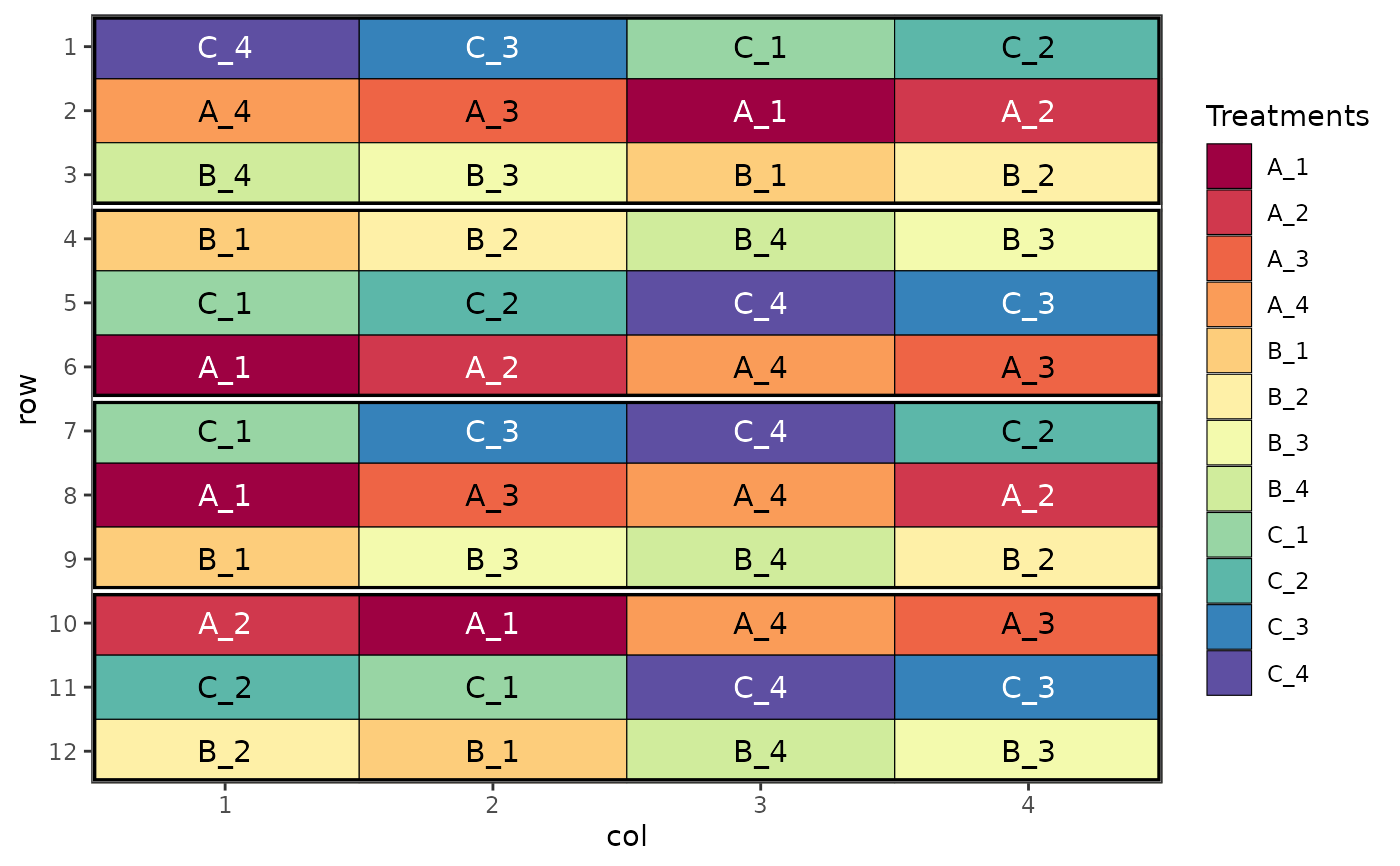
 # Strip plot design
des.out <- design(type = "strip", treatments = c("A", "B", "C"), sub_treatments = 1:4,
reps = 4, nrows = 12, ncols = 4, brows = 3, bcols = 4, seed = 42)
#> Source of Variation df
#> ==================================================
#> Block stratum 3
#> --------------------------------------------------
#> Row strip stratum
#> treatments 2
#> treatments Residual 6
#> ==================================================
#> Column strip stratum
#> sub_treatments 3
#> sub_treatments Residual 9
#> ==================================================
#> Observational unit stratum
#> treatments:sub_treatments 6
#> Interaction Residual 18
#> ==================================================
#> Total 47
# Strip plot design
des.out <- design(type = "strip", treatments = c("A", "B", "C"), sub_treatments = 1:4,
reps = 4, nrows = 12, ncols = 4, brows = 3, bcols = 4, seed = 42)
#> Source of Variation df
#> ==================================================
#> Block stratum 3
#> --------------------------------------------------
#> Row strip stratum
#> treatments 2
#> treatments Residual 6
#> ==================================================
#> Column strip stratum
#> sub_treatments 3
#> sub_treatments Residual 9
#> ==================================================
#> Observational unit stratum
#> treatments:sub_treatments 6
#> Interaction Residual 18
#> ==================================================
#> Total 47