Assimilative causal inference (ACI) in R

1. The question

Assimilative causal inference (Andreou, Chen and Bollt, 2026) treats causality as an inverse problem. Given a model of how an observed process x and a hidden process y evolve together, it asks whether the future of x carries information about y_t that the past of x did not. If it does, y drives x, and the amount of new information is the strength of that influence at time t. The answer is computed along one trajectory, so it describes causality as it happened rather than on average.

The causal influence range (Andreou and Chen, 2026) extends the question from strength to duration: for how long does an influence planted at time t persist, and how far back did the precursors of an event reach. This release computes the forward range.

2. The model comes first

In a regression workflow the model is the output: lm() is handed data and returns coefficients. Here the model is the input, a statement of how the observed and hidden variables evolve and how noisy each is, supplied before the question is asked. It can be a benchmark constructor such as aci_dyad_model(), the coefficient blocks written directly with aci_model(), or a full drift that aci_model_from_affine() splits for you. The closed-form ACI engine describes the three routes. Learning the model from data is not part of this release.

Two reconstructions and one number

Given the model, two Gaussian reconstructions of the hidden state are available in closed form:

• the filter p(y_t \mid x_{\le t}), what the past of x says.
• the smoother p(y_t \mid x_{\le T}), what the past and the future of x say together.

If the future sharpens the reconstruction, y influenced x. The ACI metric is the relative entropy between the two,

\mathrm{ACI}(t) = D_{\mathrm{KL}}\!\big(p^{\text{smoother}}_t \,\big\|\, p^{\text{filter}}_t\big) \ge 0,

and it splits into a signal part, from disagreement between the two means, and a dispersion part, from disagreement between the two spreads.

3. A worked example

The model comes first, so the example simulates from it and holds the hidden path aside to check the reconstruction against.

truth <- aci_dyad_model(params = list(d_x = 1, gamma = 2, f_x = 1.5, s_x = 0.7,
                                      d_y = 1, f_y = 0.5, s_y = 2))
sim <- simulate(truth, seed = 8, t_end = 5, dt = 5e-3, burn_in = 1)
dat <- data.frame(t = sim$obs$t, x1 = sim$obs$x[, 1], y = sim$hidden[, 1])
head(dat, 3)
#>       t       x1         y
#> 1 0.000 1.221123 0.4218527
#> 2 0.005 1.198887 0.4526444
#> 3 0.010 1.194724 0.5773667

The engine takes an observation object rather than a data frame, so the observed column goes through observed_trajectory(). That call is also the way in for your own data: it derives the time step from the supplied times and refuses a non-uniform grid.

ob <- observed_trajectory(dat$t, dat$x1, names = "x1")
ob
#> <obs_traj> k = 1, N+1 = 1001, dt = 0.005, span [0, 5]

Supply the model, the observations and a prior on the hidden state. aci_filter() and aci_smoother() return the two reconstructions, and aci() runs the pair and scores every time point.

init <- list(mean = 0, cov = matrix(1, 1, 1))
filt <- aci_filter(truth, ob, init = init)
smoo <- aci_smoother(truth, ob, filter = filt)
res  <- aci(truth, ob, init = init)

Name the prior. Omitting cov falls back to a diffuse prior with a warning, and the opening steps of such a run show the prior washing out rather than anything causal.

4. Read the result

plot(smoo, truth = dat$y)
legend("topright", c("reconstruction, two standard deviations", "withheld truth"),
       col = c(1, 2), lty = 1, bty = "n")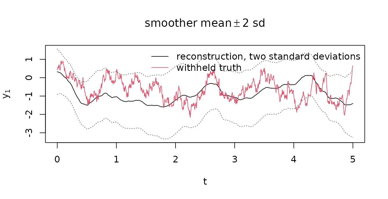

The smoother’s reconstruction of the hidden path with a band of two standard deviations, against the path that was withheld.

plot(res)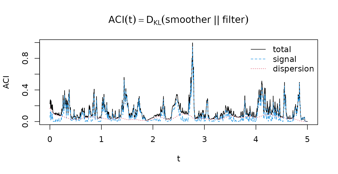

The ACI metric along the record, with its signal and dispersion parts.

print() reports the peak of the metric and where it fell:

res
#> <aci_result> engine = cgns | peak ACI = 0.9968 at t = 2.77

5. The influence range

For how long does y influence x_1? aci_range() answers per anchor time:

fc <- aci_range(res, anchors = seq(1L, length(ob$t), by = 25L))
#> Warning in .forward_cir_compiled(bundle, filter = x$paths$filter, init =
#> x$handles$init, : 1 forward CIR values masked (M < 1e-05); interpret CIRs
#> jointly with the ACI metric (Andreou & Chen 2026, Remark B.4).
fc
#> <cir_result> forward | method = exact (objective_on_truncated_table) | masked/NA: 1 of 41
#>   status: resolved 20, censored 20, insufficient 1
head(data.frame(t = fc$t, tau = fc$tau, M = fc$M, status = fc$status), 4)
#>       t        tau         M   status
#> 1 0.000 0.05790157 0.2617151 resolved
#> 2 0.125 0.11452837 0.1107143 resolved
#> 3 0.250 0.07026236 0.3480466 resolved
#> 4 0.375 0.03668586 0.4332652 resolved
plot(fc)

The forward causal influence range at the reported anchor times.

Each row is one anchor time t. tau is the range in the model’s time units and M is the peak finite-lag divergence there. anchors chooses which anchor times are reported, and only those rows are formed, which matters because forming every row of a long record is quadratic work.

An anchor whose peak divergence is too small to divide by is masked rather than reported as an inflated length, and the warning above says how many. status carries that reading and three others:

table(fc$status)
#> 
#>        resolved        censored below_threshold    insufficient 
#>              20              20               0               1

Here 20 of the 41 anchors come back censored, a property of a short record rather than of the model: after an anchor late in a five-unit series there is not always enough future left to resolve the influence it planted, and a censored range is a lower bound. The decline of the range at the end of the plot is the same finite-record effect. The closed-form ACI engine gives the full status vocabulary and the conventions each number is computed under.

6. Scope of this release

What is here is the closed-form engine: models in the conditional Gaussian nonlinear system (CGNS) class, for which the filter, the smoother and the metric have exact solutions, and the forward influence range. Learning the dynamics from data, the backward range, significance testing and the ensemble engine for systems outside the class are not in this release.

The closed-form ACI engine (vignette("vignette-2-advanced")) documents the machinery and its arguments. Reproducing the reference MATLAB codebase (vignette("vignette-3-matlab")) states which numbers of the authors’ implementation this package reproduces, and under which conventions. ?aci_references lists the sources.

References

Andreou, M., Chen, N. and Bollt, E. (2026). Assimilative causal inference. Nature Communications, 17, 1854. doi:10.1038/s41467-026-68568-0

Andreou, M. and Chen, N. (2026). Bridging prediction and attribution: identifying forward and backward causal influence ranges using assimilative causal inference. arXiv:2510.21889. doi:10.48550/arXiv.2510.21889