Multiple Comparison Tests — mct.out • BiometryTraining

A function for comparing and ranking predicted means with Tukey's Honest Significant Difference (HSD) Test.

Usage

mct.out(
  model.obj,
  pred.obj,
  classify,
  sig = 0.05,
  int.type = "ci",
  trans = NA,
  offset = NA,
  decimals = 2,
  order = "default",
  plot = FALSE,
  label_height = 0.1,
  rotation = 0,
  save = FALSE,
  savename = "predicted_values",
  pred
)

Arguments

model.obj: An ASReml-R or aov model object. Will likely also work with lme (nlme::lme()), lmerMod (lme4::lmer()) models as well.
pred.obj: An ASReml-R prediction object with sed = TRUE. Not required for other models, so set to NA.
classify: Name of predictor variable as string.
sig: The significance level, numeric between 0 and 1. Default is 0.05.
int.type: The type of confidence interval to calculate. One of ci, 1se or 2se. Default is ci.
trans: Transformation that was applied to the response variable. One of log, sqrt, logit or inverse. Default is NA.
offset: Numeric offset applied to response variable prior to transformation. Default is NA. Use 0 if no offset was applied to the transformed data. See Details for more information.
decimals: Controls rounding of decimal places in output. Default is 2 decimal places.
order: Order of the letters in the groups output. Options are 'default', 'ascending' or 'descending'. Alternative options that are accepted are increasing and decreasing. Partial matching of text is performed, allowing entry of 'desc' for example.
plot: Automatically produce a plot of the output of the multiple comparison test? Default is FALSE. This is maintained for backwards compatibility, but the preferred method now is to use autoplot(<mct.out output>). See autoplot.mct() for more details.
label_height: Height of the text labels above the upper error bar on the plot. Default is 0.1 (10%) of the difference between upper and lower error bars above the top error bar.
rotation: Rotate the text output as Treatments within the plot. Allows for easier reading of long treatment labels. Number between 0 and 360 (inclusive) - default 0
save: Logical (default FALSE). Save the predicted values to a csv file?
savename: A file name for the predicted values to be saved to. Default is predicted_values.
pred: Deprecated. Use classify instead.

Value

A list containing a data frame with predicted means, standard errors, confidence interval upper and lower bounds, and significant group allocations (named predicted_values), as well as a plot visually displaying the predicted values (named predicted_plot). If some of the predicted values are aliased, a warning is printed, and the aliased treatment levels are returned in the output (named aliased).

Details

Some transformations require that data has a small offset applied, otherwise it will cause errors (for example taking a log of 0, or square root of negative values). In order to correctly reverse this offset, if the trans argument is supplied, an offset value must also be supplied. If there was no offset required for a transformation, then use a value of 0 for the offset argument.

References

Jørgensen, E. & Pedersen, A. R. How to Obtain Those Nasty Standard Errors From Transformed Data - and Why They Should Not Be Used. http://citeseerx.ist.psu.edu/viewdoc/summary?doi=10.1.1.47.9023

Examples

# Fit aov model
model <- aov(Petal.Length ~ Species, data = iris)

# Display the ANOVA table for the model
anova(model)
#> Analysis of Variance Table
#> 
#> Response: Petal.Length
#>            Df Sum Sq Mean Sq F value    Pr(>F)    
#> Species     2 437.10 218.551  1180.2 < 2.2e-16 ***
#> Residuals 147  27.22   0.185                      
#> ---
#> Signif. codes:  0 ‘***’ 0.001 ‘**’ 0.01 ‘*’ 0.05 ‘.’ 0.1 ‘ ’ 1

# Determine ranking and groups according to Tukey's Test
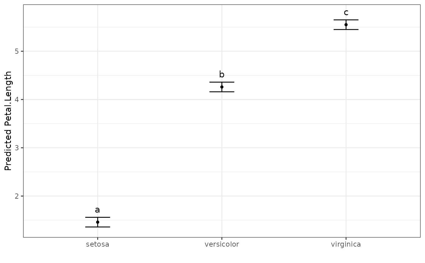
pred.out <- mct.out(model, classify = "Species")

# Display the predicted values table
pred.out
#>      Species predicted.value std.error  Df groups  ci  low   up
#> 1     setosa            1.46      0.06 147      a 0.1 1.36 1.56
#> 2 versicolor            4.26      0.06 147      b 0.1 4.16 4.36
#> 3  virginica            5.55      0.06 147      c 0.1 5.45 5.65

# Show the predicted values plot
autoplot(pred.out, label_height = 0.5)




if (FALSE) {
# ASReml-R Example
library(asreml)

#Fit ASReml Model
model.asr <- asreml(yield ~ Nitrogen + Variety + Nitrogen:Variety,
                    random = ~ Blocks + Blocks:Wplots,
                    residual = ~ units,
                    data = asreml::oats)

wald(model.asr) #Nitrogen main effect significant

#Calculate predicted means
pred.asr <- predict(model.asr, classify = "Nitrogen", sed = TRUE)

#Determine ranking and groups according to Tukey's Test
pred.out <- mct.out(model.obj = model.asr, pred.obj = pred.asr,
                    classify = "Nitrogen", order = "descending", decimals = 5)

pred.out}